Darcy friction factor formulae
In fluid dynamics, the Darcy friction factor formulae are equations – based on experimental data and theory – for the Darcy friction factor. The Darcy friction factor is a dimensionless quantity used in the Darcy–Weisbach equation, for the description of friction losses in pipe flow as well as open channel flow. It is also known as the Darcy–Weisbach friction factor or Moody friction factor and is four times larger than the Fanning friction factor.[1]
Flow regime
Which friction factor formula may be applicable depends upon the type of flow that exists:
- Laminar flow
- Transition between laminar and turbulent flow
- Fully turbulent flow in smooth conduits
- Fully turbulent flow in rough conduits
- Free surface flow.
Laminar flow
The Darcy friction factor for laminar flow in a circular pipe (Reynolds number less than 2320) is given by the following formula:

where:
-
 is the Darcy friction factor
 -
 is the Reynolds number.
Transition flow
Transition (neither fully laminar nor fully turbulent) flow occurs in the range of Reynolds numbers between 2300 and 4000. The value of the Darcy friction factor may be subject to large uncertainties in this flow regime.
Turbulent flow in smooth conduits
The Blasius correlation is the simplest equation for computing the Darcy friction factor. Because the Blasius correlation has no term for pipe roughness, it is valid only to smooth pipes. However, the Blasius correlation is sometimes used in rough pipes because of its simplicity. The Blasius correlation is valid up to the Reynolds number 100000.
Turbulent flow in rough conduits
The Darcy friction factor for fully turbulent flow (Reynolds number greater than 4000) in rough conduits is given by the Colebrook equation.
Free surface flow
The last formula in the Colebrook equation section of this article is for free surface flow. The approximations elsewhere in this article are not applicable for this type of flow.
Choosing a formula
Before choosing a formula it is worth knowing that in the paper on the Moody chart, Moody stated the accuracy is about ±5% for smooth pipes and ±10% for rough pipes. If more than one formula is applicable in the flow regime under consideration, the choice of formula may be influenced by one or more of the following:
- Required precision
- Speed of computation required
- Available computational technology:
- calculator (minimize keystrokes)
- spreadsheet (single-cell formula)
- programming/scripting language (subroutine).
Compact forms
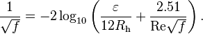
The Colebrook equation is an implicit equation that combines experimental results of studies of turbulent flow in smooth and rough pipes. It was developed in 1939 by C. F. Colebrook.[2] The 1937 paper by C. F. Colebrook and C. M. White[3] is often erroneously cited as the source of the equation. This is partly because Colebrook in a footnote (from his 1939 paper) acknowledges his debt to White for suggesting the mathematical method by which the smooth and rough pipe correlations could be combined. The equation is used to iteratively solve for the Darcy–Weisbach friction factor f. This equation is also known as the Colebrook–White equation.
For conduits that are flowing completely full of fluid at Reynolds numbers greater than 4000, it is defined as:
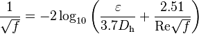
- or
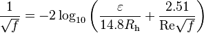
where:
- is the Darcy friction factor
- Roughness height,
 (m, ft)
 - Hydraulic diameter,
 (m, ft) – For fluid-filled, circular conduits, = D = inside diameter
 - Hydraulic radius,
 (m, ft) – For fluid-filled, circular conduits, = D/4 = (inside diameter)/4
 - is the Reynolds number
- How to check the ? Compute both sides of the Colebrook-White equation with the and if both sides are the same then the was good.
Note: Some sources use a constant of 3.71 in the denominator for the roughness term in the first equation above.[4]
Solving
The Colebrook equation is usually solved numerically due to its implicit nature. Recently, the Lambert W function has been employed to obtain explicit reformulation of the Colebrook equation.[5]
You can solve the Colebrook equation by iteration using the Newton–Raphson method. An example is provided in C# here.[6]
The Easy and True solution to compute the f is not hard in Excel because the Log makes a number smaller. Change the 1/sqrt(f) to X. On the right side the 2.51/(Re*sqrt(f)) can be re-written to 2.51/Re*X. Then the easy equation will be X=-2*Log(Rr/3.7+2.51*X/Re).
In Excel, type a GUESS number. Then below the GUESS number type =-2*Log(Rr/3.7+2.51/Re*X). Also enter the Rr and Re numbers and for the X, just point the GUESS number. Then the format cell below the GUESS, format the cell to at least 16 digits. Next, copy the cell below the GUESS to about 20 cells below the GUESS (For each row the X will be the previous number). You will see the cells soon stop changing. Then enter the cell below the bottom cell to =1/X/X, but for the X's just point to the previous cell, also format that cell to 16 digits.
This will be the right f number. Then to test it, type two more cells, First type =1/Sqrt(f), Second type =-2*Log(Rr/3.7+2.51/(Re*sqrt(f))), for the f, just point to the f, computed as 1/X/X. And format them both to at least 16 digits. They both should be the X you solved. But it the last digits are off a little bit, then Excel missed rounding the last digits.
You can save the Excel program, and next just change the Rr and Re numbers below the GUESS and copy that cell to just before the =1/X/X. The best GUESS is about 3 to 10. If you Guess 100 or 1000 it might need one more loop out of the 20 loops. A Guess from 0 to 10 might save one loop. The other numbers in the Log, other than X, will save some loops.
If you can make a VBA in Excel, here is a quick VBA ...(The "Static Function Log10(X)" below is and extra Excel's function that makes Log(10), not just a Log.)
Function Easy(Rr As Double, Re As Double) As Double
   Dim A As Double, B As Double, D As Double, X As Double, F As Double, L As Integer
   D = 3 : A = 2.51 / Re: B = Rr / 3.7
   While X <> D
           X = -2 * Log10(B + A * D)
           D = -2 * Log10(B + A * X)
           L = L + 1: If L > 20 Then X = D '... more than 20 loops, Excel can not compute more digits.
   Wend
   F = 1 / X / X
   Easy = F
End Function
Static Function Log10(X)
Log10 = Log(X) / Log(10#)
End Function
In Excel just enter this "=Easy(Rr,Re)" for the Excel's VBA, enter the right Rr and Re numbers. Went you compute the correct numbers, you may learn that "Goudar–Sonnad" is very close, but sometimes it is off some, and "Serghides's solution" is right sometimes, but most of the others are always wrong to many digits.
My first training was that if an X is on both sides of an equation, but one side in it a Log, then the X can be solved. Example X=Log(X)+10 and the Log makes the X much closer per loop. If you guess a number of 100 the first loop is 12, and if you guess 1000, the first loop is 13. If your program can compute 100 digits,it might take 30 loops to get 100 correct digits.
Also, do you know that there are six different versions of the Colebrook-White equations? Below are the six different equations that be can solved like the Ease and True solution. The first is the main one, but the others are very close to the main one.
X=-2*Log(Rr/3.7+2.51/Re*X) ____________________ :X=1.74-2*Log(2*Rr+18.7/Re*X)
X=1.14+2*Log(1/Rr)-2*Log(1+(9.3/(Re*Rr)*X)) ______ :X=1.14-2*Log(Rr+9.35/Re*X)
X=-2*Log(Rr/3.71+2.51/Re*X) ___________________ :X=-2*Log(Rr/3.72+2.51/Re*X)
Expanded forms
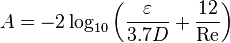
Additional, mathematically equivalent forms of the Colebrook equation are:
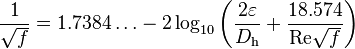
- where:
- 1.7384... = 2 log (2 × 3.7) = 2 log (7.4)
- 18.574 = 2.51 × 3.7 × 2
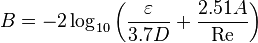
- where:
and

- or
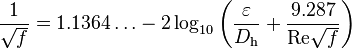
- where:
- 1.1364... = 1.7384... − 2 log (2) = 2 log (7.4) − 2 log (2) = 2 log (3.7)
- 9.287 = 18.574 / 2 = 2.51 × 3.7.
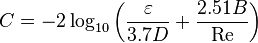
- where:
The additional equivalent forms above assume that the constants 3.7 and 2.51 in the formula at the top of this section are exact. The constants are probably values which were rounded by Colebrook during his curve fitting; but they are effectively treated as exact when comparing (to several decimal places) results from explicit formulae (such as those found elsewhere in this article) to the friction factor computed via Colebrook's implicit equation.
Equations similar to the additional forms above (with the constants rounded to fewer decimal places, or perhaps shifted slightly to minimize overall rounding errors) may be found in various references. It may be helpful to note that they are essentially the same equation.
Free surface flow
Another form of the Colebrook-White equation exists for free surfaces. Such a condition may exist in a pipe that is flowing partially full of fluid. For free surface flow:
Approximations of the Colebrook equation
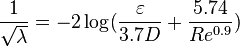
Haaland equation
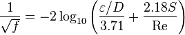
The Haaland equation was proposed by Norwegian Institute of Technology professor Haaland in 1984. It is used to solve directly for the Darcy–Weisbach friction factor f for a full-flowing circular pipe. It is an approximation of the implicit Colebrook–White equation, but the discrepancy from experimental data is well within the accuracy of the data. It was developed by S. E. Haaland in 1983.
The Haaland equation is defined as:
![\frac{1}{\sqrt {f}} = -1.8 \log_{10} \left[ \left( \frac{\varepsilon/D}{3.7} \right)^{1.11} + \frac{6.9}{\mathrm{Re}} \right]](../I/m/91bd810a870ee7d50c46ca4f7264caf2.png)
where:
- is the Darcy friction factor
-
 is the relative roughness
 - is the Reynolds number.
Swamee–Jain equation
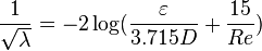
The Swamee–Jain equation is used to solve directly for the Darcy–Weisbach friction factor f for a full-flowing circular pipe. It is an approximation of the implicit Colebrook–White equation.
![f = 0.25 \left[\log_{10} \left(\frac{\varepsilon}{3.7D} + \frac{5.74}{\mathrm{Re}^{0.9}}\right)\right]^{-2}](../I/m/dd859a547bf48115b73c2e14c62b725f.png)
where f is a function of:
- Roughness height, ε (m, ft)
- Pipe diameter, D (m, ft)
- Reynolds number, Re (unitless).
Serghides's solution
Serghides's solution is used to solve directly for the Darcy–Weisbach friction factor f for a full-flowing circular pipe. It is an approximation of the implicit Colebrook–White equation. It was derived using Steffensen's method.[9]
The solution involves calculating three intermediate values and then substituting those values into a final equation.
where f is a function of:
- Roughness height, ε (m, ft)
- Pipe diameter, D (m, ft)
- Reynolds number, Re (unitless).
The equation was found to match the Colebrook–White equation within 0.0023% for a test set with a 70-point matrix consisting of ten relative roughness values (in the range 0.00004 to 0.05) by seven Reynolds numbers (2500 to 108).
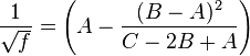
Goudar–Sonnad equation
Goudar equation is the most accurate approximation to solve directly for the Darcy–Weisbach friction factor f for a full-flowing circular pipe. It is an approximation of the implicit Colebrook–White equation. Equation has the following form[10]


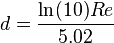
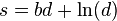

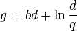

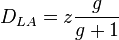
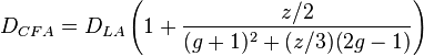
![\frac{1}{\sqrt {f}} = {a\left[ \ln\left( \frac{d}{q} \right) + D_{CFA} \right] }](../I/m/3bfe2993ed08d87e993d04e4deecd0a6.png)
where f is a function of:
- Roughness height, ε (m, ft)
- Pipe diameter, D (m, ft)
- Reynolds number, Re (unitless).
Brkić solution
Brkić shows one approximation of the Colebrook equation based on the Lambert W-function[11]
where Darcy friction factor f is a function of:
- Roughness height, ε (m, ft)
- Pipe diameter, D (m, ft)
- Reynolds number, Re (unitless).
The equation was found to match the Colebrook–White equation within 3.15%.
Blasius correlations
Early approximations by Paul Richard Heinrich Blasius in terms of the Moody friction factor are given in one article of 1913:[12]
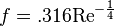 .
.
Johann Nikuradse in 1932 proposed that this corresponds to a power law correlation for the fluid velocity profile.
Mishra and Gupta in 1979 proposed a correction for curved or helically coiled tubes, taking into account the equivalent curve radius, Rc:[13]
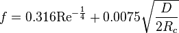 ,
,
with,
![R_c = R\left[1 + \left(\frac{H}{2 \pi R} \right)^2\right]](../I/m/613451a5b95dc0fb4d2044285e8731bc.png)
where f is a function of:
- Pipe diameter, D (m, ft)
- Curve radius, R (m, ft)
- Helicoidal pitch, H (m, ft)
- Reynolds number, Re (unitless)
valid for:
- Retr < Re < 105
- 6.7 < 2Rc/D < 346.0
- 0 < H/D < 25.4
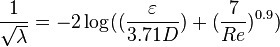
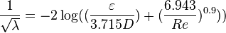
Table of Approximations
The following table lists historical approximations where:[14]
- Re, Reynolds number (unitless);
- λ, Darcy friction factor (dimensionless);
- ε, roughness of the inner surface of the pipe (dimension of length);
- D, inner pipe diameter;
-
 is the base-10 logarithm.
Note that the Churchill equation [15] (1977) is the only one that returns a correct value for friction factor in the laminar flow region (Reynolds number < 2300). All of the others are for transitional and turbulent flow only.
| Equation | Author | Year | Ref |
|---|---|---|---|
|
|
Moody | 1947 | |
|
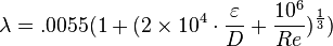
|
Wood | 1966 | |
|
|
Eck | 1973 | |
|
|
Jain and Swamee | 1976 | |
|
|
Churchill | 1973 | |
|
|
Jain | 1976 | |
|
|
Churchill | 1977 | |
|
|
Chen | 1979 | |
|
|
Round | 1980 | |
|
|
Barr | 1981 | |
|
|
Zigrang and Sylvester | 1982 | |
|
|
Haaland[lower-alpha 1][7] | 1983 | |
|
|
Serghides | 1984 | |
|
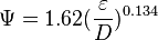
|
Manadilli | 1997 | |
|
|
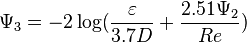
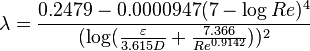
Monzon, Romeo, Royo | 2002 | |
|
|
Goudar, Sonnad | 2006 | |
|
|
Vatankhah, Kouchakzadeh | 2008 | |
|
|
Buzzelli | 2008 | |
|
|
Avci, Kargoz | 2009 | |
|
|
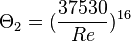
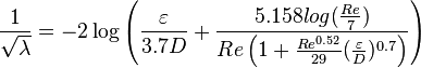
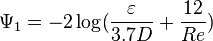
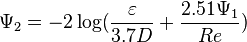
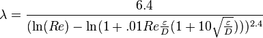
Evangleids, Papaevangelou, Tzimopoulos | 2010 |

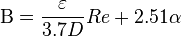
![\lambda = 8[(\frac{8}{Re})^{12} + \frac{1}{(\Theta_1 + \Theta_2)^{1.5}})]^{\frac{1}{12}}](../I/m/bf30e56931699dd9e0122011aac798c2.png)
![\Theta_1=[-2.457 \ln[(\frac{7}{Re})^{0.9} + 0.27\frac{\varepsilon}{D}]]^{16}](../I/m/e4797250ee9fcdd3e2d803d74ca44029.png)
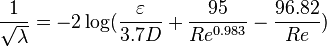
![\frac{1}{\sqrt{\lambda}} = -2 \log [\frac{\varepsilon}{3.7065D} - \frac{5.0452}{Re} \log(\frac{1}{2.8257}(\frac{\varepsilon}{D})^{1.1098} + \frac{5.8506}{Re^{0.8981}})]](../I/m/c5b59fadca29f36d38f802e08b6399a5.png)
![\frac{1}{\sqrt{\lambda}} = 1.8\log[\frac{Re}{0.135Re(\frac{\varepsilon}{D}) +6.5}]](../I/m/999775b9a959d7add269dea10803308d.png)
![\frac{1}{\sqrt{\lambda}} = -2 \log [\frac{\varepsilon}{3.7D} - \frac{5.02}{Re} \log(\frac{\varepsilon}{3.7D} - \frac{5.02}{Re} \log(\frac{\varepsilon}{3.7D} + \frac{13}{Re}))]](../I/m/251464b09e6ff3bc49975e8f9b71f9cc.png)
![\frac{1}{\sqrt{\lambda}} = -2 \log [\frac{\varepsilon}{3.7D} - \frac{5.02}{Re} \log(\frac{\varepsilon}{3.7D} + \frac{13}{Re})]](../I/m/27294617af6e3eb3d9c92817bb541ff8.png)
![\frac{1}{\sqrt{\lambda}} = -1.8 \log \left[\left(\frac{\varepsilon}{3.7D}\right)^{1.11} + \frac{6.9}{Re}\right]](../I/m/33ed5f84d2f7cf9f290c8bd88e69d8e5.png)
![\lambda = [\Psi_1 - \frac{(\Psi_2-\Psi_1)^{2}}{\Psi_3-2\Psi_2+\Psi_1}]^{-2}](../I/m/80ecb45b9bc99b7553a9f5ffadbceb50.png)
![\lambda = [4.781 - \frac{(\Psi_1-4.781)^{2}}{\Psi_2-2\Psi_1+4.781}]^{-2}](../I/m/5858f53d20e5e24cdbdd83ffb7573cef.png)
![\frac{1}{\sqrt{\lambda}} = -2 \log \lbrace \frac{\varepsilon}{3.7065D}-\frac{5.0272}{Re}\log[\frac{\varepsilon}{3.827D} - \frac{4.657}{Re} \log ((\frac{\varepsilon}{7.7918D})^{0.9924} + (\frac{5.3326}{208.815 + Re})^{0.9345})] \rbrace](../I/m/2bcce7aafbf9bff9053b0e7c308614ef.png)
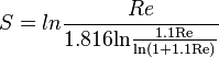
![\frac{1}{\sqrt{\lambda}} = 0.8686 \ln[\frac{0.4587Re}{(S-0.31)^{\frac{S}{(S+1)}}}]](../I/m/43070680d1665ede1de6f1281867ae63.png)
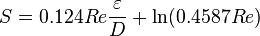
![\frac{1}{\sqrt{\lambda}} = 0.8686 \ln[\frac{0.4587Re}{(S-0.31)^{\frac{S}{(S+0.9633)}}}]](../I/m/f602d7f36407cdf8fe5fa2107103a744.png)
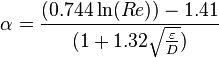
![\frac{1}{\sqrt{\lambda}} = \alpha - [ \frac {\alpha + 2\log(\frac{\Beta}{Re})}{1 + \frac{2.18}{\Beta}}]](../I/m/441df1e8b9aaae11ebb0febd74f24da1.png)
- ↑ The Haaland equation was proposed by Norwegian Institute of Technology professor Haaland in 1984. It is used to solve directly for the Darcy–Weisbach friction factor f for a full-flowing circular pipe. It is an approximation of the implicit Colebrook–White equation, but the discrepancy from experimental data is well within the accuracy of the data. It was developed by S. E. Haaland in 1983.
References
- ↑ Manning, Francis S.; Thompson, Richard E. (1991). Oilfield Processing of Petroleum. Vol. 1: Natural Gas. PennWell Books. ISBN 0-87814-343-2., 420 pages. See page 293.
- ↑ Colebrook, C.F. (February 1939). "Turbulent flow in pipes, with particular reference to the transition region between smooth and rough pipe laws". Journal of the Institution of Civil Engineers (London).
- ↑ Colebrook, C. F. and White, C. M. (1937). "Experiments with Fluid Friction in Roughened Pipes". Proceedings of the Royal Society of London. Series A, Mathematical and Physical Sciences 161 (906): 367–381. Bibcode:1937RSPSA.161..367C. doi:10.1098/rspa.1937.0150.
- ↑ VDI Heat Atlas second edition page 1058 (ISBN 978-3-540-77876-9)
- ↑ More, A. A. (2006). "Analytical solutions for the Colebrook and White equation and for pressure drop in ideal gas flow in pipes". Chemical Engineering Science 61 (16): 5515–5519. doi:10.1016/j.ces.2006.04.003.
- ↑ Métodos Numéricos con C#
- ↑ 7.0 7.1 BS Massey Mechanics of Fluids 6th Ed ISBN 0-412-34280-4
- ↑ P.K. Swami, A.K. Jaine, Explicit equations for pipeflow problems, J Hydraulics Div, Proc ASCE (1976), pp. 657–664 May
- ↑ Serghides, T.K (1984). "Estimate friction factor accurately". Chemical Engineering Journal 91(5): 63–64.
- ↑ Goudar, C.T., Sonnad, J.R. (August 2008). "Comparison of the iterative approximations of the Colebrook–White equation". Hydrocarbon Processing Fluid Flow and Rotating Equipment Special Report(August 2008): 79–83.
- ↑ Brkić, Dejan (2011). "An Explicit Approximation of Colebrook’s equation for fluid flow friction factor". Petroleum Science and Technology 29 (15): 1596–1602. doi:10.1080/10916461003620453.
- ↑ Trinh, On the Blasius correlation for friction factors, p. 1
- ↑ Adrian Bejan, Allan D. Kraus, Heat transfer handbook, John Wiley & Sons, 2003
- ↑ Beograd, Dejan Brkić (March 2012). "Determining Friction Factors in Turbulent Pipe Flow". Chemical Engineering: 34–39.(subscription required)
- ↑ Churchill, S.W. (November 7, 1977). "Friction-factor equation spans all fluid-flow regimes". Chemical Engineering: 91–92.
Further reading
- Colebrook, C.F. (February 1939). "Turbulent flow in pipes, with particular reference to the transition region between smooth and rough pipe laws". Journal of the Institution of Civil Engineers (London). doi:10.1680/ijoti.1939.13150.
For the section which includes the free-surface form of the equation – "Computer Applications in Hydraulic Engineering" (5th ed.). Haestad Press. 2002., p. 16. - Haaland, SE (1983). "Simple and Explicit Formulas for the Friction Factor in Turbulent Flow". Journal of Fluids Engineering (ASME) 105 (1): 89–90. doi:10.1115/1.3240948.
- Swamee, P.K.; Jain, A.K. (1976). "Explicit equations for pipe-flow problems". Journal of the Hydraulics Division (ASCE) 102 (5): 657–664.
- Serghides, T.K (1984). "Estimate friction factor accurately". Chemical Engineering 91 (5): 63–64. – Serghides' solution is also mentioned here.
- Moody, L.F. (1944). "Friction Factors for Pipe Flow". Transactions of the ASME 66 (8): 671–684.
- Brkić, Dejan (2011). "Review of explicit approximations to the Colebrook relation for flow friction". Journal of Petroleum Science and Engineering 77 (1): 34–48. doi:10.1016/j.petrol.2011.02.006.
- Brkić, Dejan (2011). "W solutions of the CW equation for flow friction". Applied Mathematics Letters 24 (8): 1379–1383. doi:10.1016/j.aml.2011.03.014.
- Geron, Harrell (2010, but Russia told me they wanted to pay for the Easy Solution, but they wanted to own it so they could sell it to the world engineers, I said, "No, I want all world users to get it for free."). "Easy and True solutions". Applied 6 different version add... http://colebrook-white.blogspot.com/''. Check date values in:
|date=(help)