Cylindrical multipole moments
Cylindrical multipole moments are the coefficients in a series expansion of a potential that varies logarithmically with the distance to a source, i.e., as  . Such potentials arise in the electric potential of long line charges, and the analogous sources for the magnetic potential and gravitational potential.
For clarity, we illustrate the expansion for a single line charge, then generalize to an arbitrary distribution of line charges. Through this article, the primed coordinates such
as  refer to the position of the line charge(s), whereas the unprimed coordinates such as
  refer to the point at which the potential is being observed. We use cylindrical coordinates throughout, e.g., an arbitrary vector
  has coordinates
  where
where  is the radius from the
  axis,
axis,  is the azimuthal angle and is the normal Cartesian coordinate. By assumption, the line charges are infinitely long and aligned with the axis.
Cylindrical multipole moments of a line charge
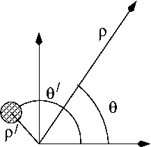
The electric potential of a line charge  located at is given by

where  is the shortest distance between the line charge and the observation point.
By symmetry, the electric potential of an infinite linecharge has no -dependence. The line charge is the charge per unit length in the
-direction, and has units of (charge/length). If the radius of the observation point is greater than the radius  of the line charge, we may factor out
and expand the logarithms in powers of 
![\Phi(\rho, \theta) =
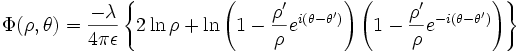
\frac{-\lambda}{2\pi\epsilon} \left\{\ln \rho -
\sum_{k=1}^{\infty} \left( \frac{1}{k} \right) \left( \frac{\rho^{\prime}}{\rho} \right)^{k}
\left[ \cos k\theta \cos k\theta^{\prime} + \sin k\theta \sin k\theta^{\prime} \right] \right\}](../I/m/d4277aca82a34e679dcd152dd12b13c3.png)
which may be written as
where the multipole moments are defined as

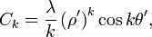
and
Conversely, if the radius of the observation point is less than the radius of the line charge, we may factor out  and expand the logarithms in powers of
![\Phi(\rho, \theta) =
\frac{-\lambda}{2\pi\epsilon} \left\{\ln \rho^{\prime} -
\sum_{k=1}^{\infty} \left( \frac{1}{k} \right) \left( \frac{\rho}{\rho^{\prime}} \right)^{k}
\left[ \cos k\theta \cos k\theta^{\prime} + \sin k\theta \sin k\theta^{\prime} \right] \right\}](../I/m/ad604aa69eef71a1ff0811bac73a1596.png)
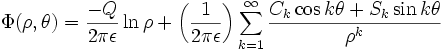
which may be written as
![\Phi(\rho, \theta) =
\frac{-Q}{2\pi\epsilon} \ln \rho^{\prime} +
\left( \frac{1}{2\pi\epsilon} \right) \sum_{k=1}^{\infty}
\rho^{k} \left[ I_{k} \cos k\theta + J_{k} \sin k\theta \right]](../I/m/41f52d3618a9aec55d4bc677af4e77ec.png)
where the interior multipole moments are defined as
and
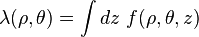
General cylindrical multipole moments
The generalization to an arbitrary distribution of line charges  is straightforward. The functional form is the same
and the moments can be written

Note that the represents the line charge per unit area in the  plane.
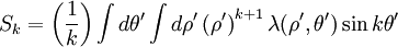
Interior cylindrical multipole moments
Similarly, the interior cylindrical multipole expansion has the functional form
where the moments are defined
![I_{k} = \left( \frac{1}{k} \right)
\int d\theta^{\prime}
\int d\rho^{\prime}
\left[ \frac{\cos k\theta^{\prime}}{\left(\rho^{\prime}\right)^{k-1}} \right]
\lambda(\rho^{\prime}, \theta^{\prime})](../I/m/27815fd3f5541f6a13c6dec0e2977692.png)
![J_{k} = \left( \frac{1}{k} \right)
\int d\theta^{\prime}
\int d\rho^{\prime}
\left[ \frac{\sin k\theta^{\prime}}{\left(\rho^{\prime}\right)^{k-1}} \right]
\lambda(\rho^{\prime}, \theta^{\prime})](../I/m/29e1052eb76d7df317e8cd829ccd1a57.png)
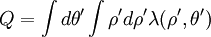
Interaction energies of cylindrical multipoles
A simple formula for the interaction energy of cylindrical multipoles (charge density 1) with a second charge density can be derived. Let  be the second charge density, and define
  as its integral over z
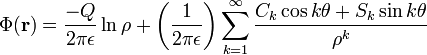
The electrostatic energy is given by the integral of the charge multiplied by the potential due to the cylindrical multipoles
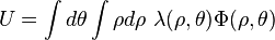
If the cylindrical multipoles are exterior, this equation becomes
![\ \ \ \ \ \ \ \ \ \ + \ \left( \frac{1}{2\pi\epsilon} \right) \sum_{k=1}^{\infty}
C_{1k} \int d\theta \int d\rho
\left[ \frac{\cos k\theta}{\rho^{k-1}} \right] \lambda(\rho, \theta)](../I/m/fb8c4a8f7e5b79d65bf1da0a2c131957.png)
![\ \ \ \ \ \ \ \ + \ \left( \frac{1}{2\pi\epsilon} \right) \sum_{k=1}^{\infty}
S_{1k} \int d\theta \int d\rho
\left[ \frac{\sin k\theta}{\rho^{k-1}} \right]
\lambda(\rho, \theta)](../I/m/c6fa699c129236ca88fc9dd97c3ec781.png)
where  ,
,  and
and  are the cylindrical multipole moments of charge distribution 1. This energy formula can be reduced to a remarkably simple form

where  and
and  are the interior cylindrical multipoles of the second charge density.
The analogous formula holds if charge density 1 is composed of interior cylindrical multipoles

where  and
and  are the interior cylindrical multipole moments of charge distribution 1, and
  and
and  are the
exterior cylindrical multipoles of the second charge density.
are the
exterior cylindrical multipoles of the second charge density.
As an example, these formulae could be used to determine the interaction energy of a small protein in the electrostatic field of a double-stranded DNA molecule; the latter is relatively straight and bears a constant linear charge density due to the phosphate groups of its backbone.