Covariant transformation

See also Covariance and contravariance of vectors

In physics, a covariant transformation is a rule (specified below) that specifies how certain entities change under a change of basis. In particular, the term is used for vectors and tensors. The transformation that describes the new basis vectors as a linear combination of the old basis vectors is defined as a covariant transformation. Conventionally, indices identifying the basis vectors are placed as lower indices and so are all entities that transform in the same way. The inverse of a covariant transformation is a contravariant transformation. Since a vector should be invariant under a change of basis, its components must transform according to the contravariant rule. Conventionally, indices identifying the components of a vector are placed as upper indices and so are all indices of entities that transform in the same way. The sum over pairwise matching indices of a product with the same lower and upper indices are invariant under a transformation.

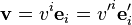
A vector itself is a geometrical quantity, in principle, independent (invariant) of the chosen basis. A vector v is given, say, in components vⁱ on a chosen basis e_i. On another basis, say e′_j, the same vector v has different components v′ⁱ and

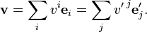
\mathbf{v} = \sum_i v^i {\mathbf e}_i = \sum_j {v'\,}^j \mathbf{e}'_j.

With v being invariant and the e_i transforming covariantly, it must be that the vⁱ (the set of numbers identifying the components) transform in a different way, being the inverse called the contravariant transformation rule.

If, for example in a 2-dimensional Euclidean space, the new basis vectors are rotated anti-clockwise with respect to the old basis vectors, then it will appear in terms of the new system that the componentwise representation of the vector was rotated in the opposite direction, i.e. clockwise (see figure).

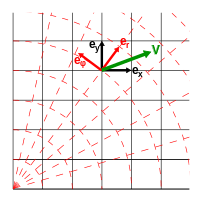
A vector v, and local tangent basis vectors {e_x,e_y} and {e_r,e_φ}.
Coordinate representations of v.

A vector v is described in a given coordinate grid (black lines) on a basis which are the tangent vectors to the (here rectangular) coordinate grid. The basis vectors are e_x and e_y. In another coordinate system (dashed and red), the new basis vectors are tangent vectors in the radial direction and perpendicular to it. These basis vectors are indicated in red as e_r and e_φ. They appear rotated anticlockwise with respect to the first basis. The covariant transformation here is thus an anticlockwise rotation.

If we view the vector v with e_φ pointed upwards, its representation in this frame appears rotated to the right. The contravariant transformation is a clockwise rotation.

Examples of covariant transformation

The derivative of a function transforms covariantly

The explicit form of a covariant transformation is best introduced with the transformation properties of the derivative of a function. Consider a scalar function f (like the temperature at a location in a space) defined on a set of points p, identifiable in a given coordinate system $x^i,\; i=0,1,\dots$ (such a collection is called a manifold). 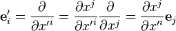If we adopt a new coordinates system ${x'}^j, j=0,1,\dots$ then for each i, the original coordinate ${x}^i$ can be expressed as a function of the new coordinates, so ${x}^i({x'}^j), j=0,1,\dots$ One can express the derivative of f in new coordinates in terms of the old coordinates, using the chain rule of the derivative, as

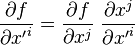
\frac{\partial f}{\partial {x'}^i} = \frac{\partial f}{\partial {x}^j} \; \frac{\partial {x}^j}{\partial {x'}^i}

This is the explicit form of the covariant transformation rule. The notation of a normal derivative with respect to the coordinates sometimes uses a comma, as follows

f_{,i} \ \stackrel{\mathrm{def}}{=}\ \frac{\partial f}{\partial x^i}

where the index i is placed as a lower index, because of the covariant transformation.

Basis vectors transform covariantly

A vector can be expressed in terms of basis vectors. For a certain coordinate system, we can choose the vectors tangent to the coordinate grid. This basis is called the coordinate basis.

To illustrate the transformation properties, consider again the set of points p, identifiable in a given coordinate system $x^i$ where $i=0,1,\dots$ (manifold). A scalar function f, that assigns a real number to every point p in this space, is a function of the coordinates $f\;(x^0,x^1,\dots)$ . A curve is a one-parameter collection of points c, say with curve parameter λ, c(λ). A tangent vector v to the curve is the derivative $dc/d\lambda$ along the curve with the derivative taken at the point p under consideration. Note that we can see the tangent vector v as an operator (the directional derivative) which can be applied to a function

{\mathbf v}[f] \ \stackrel{\mathrm{def}}{=}\ \frac{df}{d\lambda}= \frac{d\;\;}{d\lambda} f(c(\lambda))

The parallel between the tangent vector and the operator can also be worked out in coordinates

{\mathbf v}[f] = \frac{dx^i}{d\lambda} \frac{\partial f}{\partial x^i}

or in terms of operators $\partial/\partial x^i$

{\mathbf v} = \frac{dx^i}{d\lambda} \frac{\partial \;\;}{\partial x^i} = \frac{dx^i}{d\lambda} {\mathbf e}_i

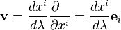
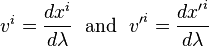
where we have written ${\mathbf e}_i = \partial/\partial x^i$ , the tangent vectors to the curves which are simply the coordinate grid itself.

If we adopt a new coordinates system ${x'}^i, \;i=0,1,\dots$ then for each i, the old coordinate ${x^i}$ can be expressed as function of the new system, so $x^i({x'}^j), j=0,1,\dots$ Let ${\mathbf e}'_i = {\partial}/{\partial {x'}^i}$ be the basis, tangent vectors in this new coordinates system. We can express ${\mathbf e}_i$ in the new system by applying the chain rule on x. As a function of coordinates we find the following transformation

{\mathbf e}'_i = \frac{\partial}{\partial {x'}^i} = \frac{\partial x^j}{\partial {x'}^i} \frac{\partial}{\partial x^j} = \frac{\partial x^j}{\partial {x'}^i} {\mathbf e}_j

which indeed is the same as the covariant transformation for the derivative of a function.

Contravariant transformation

The components of a (tangent) vector transform in a different way, called contravariant transformation. Consider a tangent vector v and call its components $v^i$ on a basis ${\mathbf e}_i$ . On another basis ${\mathbf e}'_i$ we call the components ${v'}^i$ , so

{\mathbf v} = v^i {\mathbf e}_i = {v'}^i {\mathbf e}'_i

in which

v^i = \frac{dx^i}{d\lambda} \;\mbox{ and }\; {v'}^i = \frac{d{x'}^i}{d\lambda}

If we express the new components in terms of the old ones, then

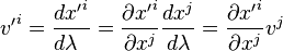
{v'}^i = \frac{d{x'}^i}{d\lambda\;\;} = \frac{\partial {x'}^i}{\partial x^j} \frac{dx^j}{d\lambda} = \frac{\partial {x'}^i}{\partial x^j} {v}^j

This is the explicit form of a transformation called the contravariant transformation and we note that it is different and just the inverse of the covariant rule. In order to distinguish them from the covariant (tangent) vectors, the index is placed on top.

Differential forms transform contravariantly

An example of a contravariant transformation is given by a differential form df. For f as a function of coordinates $x^i$ , df can be expressed in terms of $dx^i$ . The differentials dx transform according to the contravariant rule since

d{x'}^i = \frac{\partial {x'}^i}{\partial {x}^j} {dx}^j

Dual properties

Entities that transform covariantly (like basis vectors) and the ones that transform contravariantly (like components of a vector and differential forms) are "almost the same" and yet they are different. They have "dual" properties. What is behind this, is mathematically known as the dual space that always goes together with a given linear vector space.

Take any vector space T. A function f on T is called linear if, for any vectors v, w and scalar α:

f({\mathbf v}+{\mathbf w}) = f({\mathbf v}) + f({\mathbf w})

f(\alpha {\mathbf v}) = \alpha f({\mathbf v})

A simple example is the function which assigns a vector the value of one of its components (called a projection function). It has a vector as argument and assigns a real number, the value of a component.

All such scalar-valued linear functions together form a vector space, called the dual space of T. The sum f+g is again a linear function for linear f and g, and the same holds for scalar multiplication αf.

Given a basis ${\mathbf e}_i$ for T, we can define a basis, called the dual basis for the dual space in a natural way by taking the set of linear functions mentioned above: the projection functions. Each projection function (indexed by ω) produces the number 1 when applied to one of the basis vectors ${\mathbf e}_i$ . For example ${\omega}^0$ gives a 1 on ${\mathbf e}_0$ and zero elsewhere. Applying this linear function ${\omega}^0$ to a vector ${\mathbf v} =v^i {\mathbf e}_i$ , gives (using its linearity)

\omega^0({\mathbf v}) = \omega^0(v^i {\mathbf e}_i) = v^i \omega^0({\mathbf e}_i) = v^0

so just the value of the first coordinate. For this reason it is called the projection function.

There are as many dual basis vectors $\omega^i$ as there are basis vectors ${\mathbf e}_i$ , so the dual space has the same dimension as the linear space itself. It is "almost the same space", except that the elements of the dual space (called dual vectors) transform covariantly and the elements of the tangent vector space transform contravariantly.

Sometimes an extra notation is introduced where the real value of a linear function σ on a tangent vector u is given as

\sigma [{\mathbf u}] := \langle \sigma, {\mathbf u}\rangle

where $\langle\sigma, {\mathbf u}\rangle$ is a real number. This notation emphasizes the bilinear character of the form. it is linear in σ since that is a linear function and it is linear in u since that is an element of a vector space.

Co- and contravariant tensor components

Without coordinates

A tensor of type (r,s) may be defined as a real-valued multilinear function of r dual vectors and s vectors. Since vectors and dual vectors may be defined without dependence on a coordinate system, a tensor defined in this way is independent of the choice of a coordinate system.

The notation of a tensor is

T(\sigma, \ldots ,\rho, {\mathbf u}, \ldots, {\mathbf v}) \;\text{ or as }\; { T^{\sigma \ldots \rho} }_{ {\mathbf u} \ldots {\mathbf v}}

for dual vectors (differential forms) ρ, σ and tangent vectors ${\mathbf u}, {\mathbf v}$ . In the second notation the distinction between vectors and differential forms is more obvious.

With coordinates

Because a tensor depends linearly on its arguments, it is completely determined if one knows the values on a basis $\omega^i \ldots \omega^j$ and ${\mathbf e}_k \ldots {\mathbf e}_l$

T(\omega^i,\ldots,\omega^j, {\mathbf e}_k \ldots {\mathbf e}_l) = {T^{i\ldots j}}_{k\ldots l}

The numbers ${T^{i\ldots j}}_{k\ldots l}$ are called the components of the tensor on the chosen basis.

If we choose another basis (which are a linear combination of the original basis), we can use the linear properties of the tensor and we will find that the tensor components in the upper indices transform as dual vectors (so contravariant), whereas the lower indices will transform as the basis of tangent vectors and are thus covariant. For a tensor of rank 2, we can verify that

{A'}_{i j} = \frac{\partial x^l}{\partial {x'}^i} \frac{\partial x^m}{\partial {x'}^j} A_{l m}

covariant tensor

{A'\,}^{i j} = \frac{\partial {x'}^i}{\partial x^l} \frac{\partial {x'}^j}{\partial x^m} A^{l m}

contravariant tensor

For a mixed co- and contravariant tensor of rank 2

{A'\,}^i{}_j= \frac {\partial {x'}^i} {\partial x^l} \frac {\partial x^m} {\partial {x'}^j} A^l{}_m

mixed co- and contravariant tensor