Cournot competition

Cournot competition is an economic model used to describe an industry structure in which companies compete on the amount of output they will produce, which they decide on independently of each other and at the same time. It is named after Antoine Augustin Cournot^[1] (1801–1877) who was inspired by observing competition in a spring water duopoly. It has the following features:

There is more than one firm and all firms produce a homogeneous product, i.e. there is no product differentiation;
Firms do not cooperate, i.e. there is no collusion;
Firms have market power, i.e. each firm's output decision affects the good's price;
The number of firms is fixed;
Firms compete in quantities, and choose quantities simultaneously;
The firms are economically rational and act strategically, usually seeking to maximize profit given their competitors' decisions.

An essential assumption of this model is the "not conjecture" that each firm aims to maximize profits, based on the expectation that its own output decision will not have an effect on the decisions of its rivals. Price is a commonly known decreasing function of total output. All firms know $N$ , the total number of firms in the market, and take the output of the others as given. Each firm has a cost function $c_i(q_i)$ . Normally the cost functions are treated as common knowledge. The cost functions may be the same or different among firms. The market price is set at a level such that demand equals the total quantity produced by all firms. Each firm takes the quantity set by its competitors as a given, evaluates its residual demand, and then behaves as a monopoly.

History

“	The state of equilibrium... is therefore stable; i.e. if either of the producers, misled as to his true interest, leaves it temporarily, he will be brought back to it.	”
—Antoine Augustin Cournot, Recherches sur les Principes Mathematiques de la Theorie des Richesses (1838), translated by Bacon (1897).

Antoine Augustin Cournot (1801-1877) first outlined his theory of competition in his 1838 volume Recherches sur les Principes Mathematiques de la Theorie des Richesses as a way of describing the competition with a market for spring water dominated by two suppliers (a duopoly).^[2] The model was one of a number that Cournot set out "explicitly and with mathematical precision" in the volume.^[3] Specifically, Cournot constructed profit functions for each firm, and then used partial differentiation to construct a function representing a firm's best response for given (exogenous) output levels of the other firm(s) in the market.^[3] He then showed that a stable equilibrium occurs where these functions intersect (i.e. the simultaneous solution of the best response functions of each firm).^[3]

The consequence of this is that in equilibrium, each firm's expectations of how other firms will act are shown to be correct; when all is revealed, no firm wants to change its output decision.^[1] This idea of stability was later taken up and built upon as a description of Nash equilibria, of which Cournot equilibria are a subset.^[3]

Graphically finding the Cournot duopoly equilibrium

This section presents an analysis of the model with 2 firms and constant marginal cost.

p_1

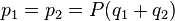
= firm 1 price,

p_2

= firm 2 price

q_1

= firm 1 quantity,

q_2

= firm 2 quantity

c

= marginal cost, identical for both firms

Equilibrium prices will be:

p_1 = p_2 = P(q_1+q_2)

This implies that firm 1’s profit is given by 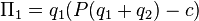$\Pi_1 = q_1(P(q_1+q_2)-c)$

Calculate firm 1’s residual demand: Suppose firm 1 believes firm 2 is producing quantity $q_2$ . What is firm 1's optimal quantity? Consider the diagram 1. If firm 1 decides not to produce anything, then price is given by 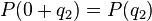$P(0+q_2)=P(q_2)$ . If firm 1 produces $q_1'$ then price is given by $P(q_1'+q_2)$ . More generally, for each quantity that firm 1 might decide to set, price is given by the curve $d_1(q_2)$ . The curve $d_1(q_2)$ is called firm 1’s residual demand; it gives all possible combinations of firm 1’s quantity and price for a given value of $q_2$ .

Determine firm 1’s optimum output: To do this we must find where marginal revenue equals marginal cost. Marginal cost (c) is assumed to be constant. Marginal revenue is a curve - $r_1(q_2)$ - with twice the slope of $d_1(q_2)$ and with the same vertical intercept. The point at which the two curves ( $c$ and $r_1(q_2)$ ) intersect corresponds to quantity $q_1''(q_2)$ . Firm 1’s optimum $q_1''(q_2)$ , depends on what it believes firm 2 is doing. To find an equilibrium, we derive firm 1’s optimum for other possible values of $q_2$ . Diagram 2 considers two possible values of $q_2$ . If $q_2=0$ , then the first firm's residual demand is effectively the market demand, $d_1(0)=D$ . The optimal solution is for firm 1 to choose the monopoly quantity; $q_1''(0)=q^m$ ( $q^m$ is monopoly quantity). If firm 2 were to choose the quantity corresponding to perfect competition, $q_2=q^c$ such that $P(q^c)=c$ , then firm 1’s optimum would be to produce nil: $q_1''(q^c)=0$ . This is the point at which marginal cost intercepts the marginal revenue corresponding to $d_1(q^c)$ .

It can be shown that, given the linear demand and constant marginal cost, the function $q_1''(q_2)$ is also linear. Because we have two points, we can draw the entire function $q_1''(q_2)$ , see diagram 3. Note the axis of the graphs has changed, The function $q_1''(q_2)$ is firm 1’s reaction function, it gives firm 1’s optimal choice for each possible choice by firm 2. In other words, it gives firm 1’s choice given what it believes firm 2 is doing.

The last stage in finding the Cournot equilibrium is to find firm 2’s reaction function. In this case it is symmetrical to firm 1’s as they have the same cost function. The equilibrium is the intersection point of the reaction curves. See diagram 4.

The prediction of the model is that the firms will choose Nash equilibrium output levels.

Calculating the equilibrium

In very general terms, let the price function for the (duopoly) industry be $P(q_1+q_2)$ and firm i have the cost structure $C_i(q_i)$ . To calculate the Nash equilibrium, the best response functions of the firms must first be calculated.

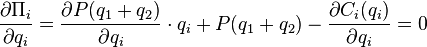
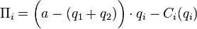
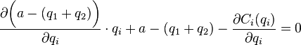
The profit of firm i is revenue minus cost. Revenue is the product of price and quantity and cost is given by the firm's cost function, so profit is (as described above): $\Pi_i = P(q_1+q_2) \cdot q_i - C_i(q_i)$ . The best response is to find the value of $q_i$ that maximises $\Pi_i$ given $q_j$ , with $i \ne j$ , i.e. given some output of the opponent firm, the output that maximises profit is found. Hence, the maximum of $\Pi_i$ with respect to $q_i$ is to be found. First take the derivative of $\Pi_i$ with respect to $q_i$ :

\frac{\partial \Pi_i }{\partial q_i} = \frac{\partial P(q_1+q_2) }{\partial q_i} \cdot q_i + P(q_1+q_2) - \frac{\partial C_i (q_i)}{\partial q_i}

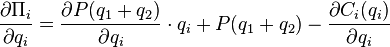
Setting this to zero for maximization:

\frac{\partial \Pi_i }{\partial q_i} = \frac{\partial P(q_1+q_2) }{\partial q_i} \cdot q_i + P(q_1+q_2) - \frac{\partial C_i (q_i)}{\partial q_i}=0

The values of $q_i$ that satisfy this equation are the best responses. The Nash equilibria are where both $q_1$ and $q_2$ are best responses given those values of $q_1$ and $q_2$ .

An example

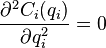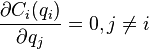Suppose the industry has the following price structure: $P(q_1+q_2)= a - (q_1+q_2)$ The profit of firm i (with cost structure $C_i(q_i)$ such that $\frac{\partial ^2C_i (q_i)}{\partial q_i^2}=0$ and $\frac{\partial C_i (q_i)}{\partial q_j}=0, j \ne i$ for ease of computation) is:

\Pi_i = \bigg(a - (q_1+q_2)\bigg) \cdot q_i - C_i(q_i)

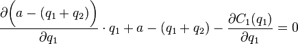
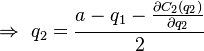
The maximization problem resolves to (from the general case):

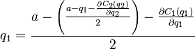
\frac{\partial \bigg(a - (q_1+q_2)\bigg) }{\partial q_i} \cdot q_i + a - (q_1+q_2) - \frac{\partial C_i (q_i)}{\partial q_i}=0

Without loss of generality, consider firm 1's problem:

\frac{\partial \bigg(a - (q_1+q_2)\bigg) }{\partial q_1} \cdot q_1 + a - (q_1+q_2) - \frac{\partial C_1 (q_1)}{\partial q_1}=0

\Rightarrow \ - q_1 + a - (q_1+q_2) - \frac{\partial C_1 (q_1)}{\partial q_1}=0

\Rightarrow \ q_1 = \frac{a - q_2 - \frac{\partial C_1 (q_1)}{\partial q_1}}{2}

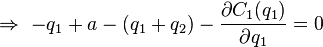
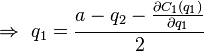
By symmetry:

\Rightarrow \ q_2 = \frac{a - q_1 - \frac{\partial C_2 (q_2)}{\partial q_2}}{2}

These are the firms' best response functions. For any value of $q_2$ , firm 1 responds best with any value of $q_1$ that satisfies the above. In Nash equilibria, both firms will be playing best responses so solving the above equations simultaneously. Substituting for $q_2$ in firm 1's best response:

\ q_1 = \frac{a - \left(\frac{a - q_1 - \frac{\partial C_2 (q_2)}{\partial q_2}}{2}\right) - \frac{\partial C_1 (q_1)}{\partial q_1}}{2}

\Rightarrow \ q_1^* = \frac{a + \frac{\partial C_2 (q_2)}{\partial q_2} - 2*\frac{\partial C_1 (q_1)}{\partial q_1}}{3}

\Rightarrow \ q_2^* = \frac{a + \frac{\partial C_1 (q_1)}{\partial q_1} - 2^*\frac{\partial C_2 (q_2)}{\partial q_2}}{3}

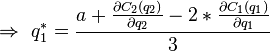
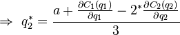
The symmetric Nash equilibrium is at $(q_1^*,q_2^*)$ . (See Holt (2005, Chapter 13) for asymmetric examples.) Making suitable assumptions for the partial derivatives (for example, assuming each firm's cost is a linear function of quantity and thus using the slope of that function in the calculation), the equilibrium quantities can be substituted in the assumed industry price structure $P(q_1+q_2)= a - (q_1+q_2)$ to obtain the equilibrium market price.

Cournot competition with many firms and the Cournot theorem

For an arbitrary number of firms, N > 1, the quantities and price can be derived in a manner analogous to that given above. With linear demand and identical, constant marginal cost the equilibrium values are as follows:

Market demand; $\ p(q)=a-bq=a-bQ=p(Q)$

Cost function; $\ c_i(q_i)=cq_i$ , for all i

\ q_i = Q/N = \frac{a-c} {b(N+1)},

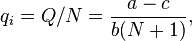
which is each individual firm's output

\sum q_i = Nq = \frac{N(a-c)} {b(N+1)},

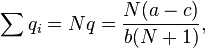
which is total industry output

\ p =a-b(Nq)= \frac{a + Nc} {N+1},

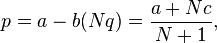
which is the market clearing price, and

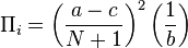\Pi_i = \left(\frac{a - c} {N+1}\right)^2 \left(\frac{1}{b}\right)

, which is each individual firm's profit.

The Cournot Theorem then states that, in absence of fixed costs of production, as the number of firms in the market, N, goes to infinity, market output, Nq, goes to the competitive level and the price converges to marginal cost.

\lim_{N\rightarrow \infty} p = c

Hence with many firms a Cournot market approximates a perfectly competitive market. This result can be generalized to the case of firms with different cost structures (under appropriate restrictions) and non-linear demand.

When the market is characterized by fixed costs of production, however, we can endogenize the number of competitors imagining that firms enter in the market until their profits are zero. In our linear example with $N$ firms, when fixed costs for each firm are $F$ , we have the endogenous number of firms:

N=\frac{a-c}{\sqrt{Fb}}-1

and a production for each firm equal to:

q=\frac{\sqrt{Fb}}{b}

This equilibrium is usually known as Cournot equilibrium with endogenous entry, or Marshall equilibrium.^[4]

Implications

Output is greater with Cournot duopoly than monopoly, but lower than perfect competition.
Price is lower with Cournot duopoly than monopoly, but not as low as with perfect competition.
According to this model the firms have an incentive to form a cartel, effectively turning the Cournot model into a Monopoly. Cartels are usually illegal, so firms might instead tacitly collude using self-imposing strategies to reduce output which, ceteris paribus will raise the price and thus increase profits for all firms involved.

Bertrand versus Cournot

Although both models have similar assumptions, they have very different implications:

Since the Bertrand model assumes that firms compete on price and not output quantity, it predicts that a duopoly is enough to push prices down to marginal cost level, meaning that a duopoly will result in perfect competition.
Neither model is necessarily "better." The accuracy of the predictions of each model will vary from industry to industry, depending on the closeness of each model to the industry situation.
If capacity and output can be easily changed, Bertrand is a better model of duopoly competition. If output and capacity are difficult to adjust, then Cournot is generally a better model.
Under some conditions the Cournot model can be recast as a two-stage model, where in the first stage firms choose capacities, and in the second they compete in Bertrand fashion.

However, as the number of firms increases towards infinity, the Cournot model gives the same result as in Bertrand model: The market price is pushed to marginal cost level.

References

↑ 1.0 1.1 Varian, Hal R. (2006), Intermediate microeconomics: a modern approach (7 ed.), W. W. Norton & Company, p. 490, ISBN 0-393-92702-4
↑ Van den Berg et al. 2011, p. 1
↑ 3.0 3.1 3.2 3.3 Morrison 1998
↑ Etro, Federico. Simple models of competition, page 6, Dept. Political Economics -- Università di Milano-Bicocca, November 2006

Holt, Charles. Games and Strategic Behavior (PDF version), PDF
Tirole, Jean. The Theory of Industrial Organization, MIT Press, 1988.
Oligoply Theory made Simple, Chapter 6 of Surfing Economics by Huw Dixon.

Topics in game theory

Definitions	Normal-form game Extensive-form game Graphical game Cooperative game Succinct game Information set Hierarchy of beliefs Preference

Equilibrium concepts	Nash equilibrium Subgame perfection Mertens-stable equilibrium Bayesian-Nash Perfect Bayesian Trembling hand Proper equilibrium Epsilon-equilibrium Correlated equilibrium Sequential equilibrium Quasi-perfect equilibrium Evolutionarily stable strategy Risk dominance Core Shapley value Pareto efficiency Quantal response equilibrium Self-confirming equilibrium Strong Nash equilibrium Markov perfect equilibrium

Strategies	Dominant strategies Pure strategy Mixed strategy Tit for tat Grim trigger Collusion Backward induction Forward induction Markov strategy

Classes of games	Symmetric game Perfect information Simultaneous game Sequential game Repeated game Signaling game Cheap talk Zero-sum game Mechanism design Bargaining problem Stochastic game n-player game Large Poisson game Nontransitive game Global games Strictly determined game

Games	Prisoner's dilemma Traveler's dilemma Coordination game Chicken Centipede game Volunteer's dilemma Dollar auction Battle of the sexes Stag hunt Matching pennies Ultimatum game Rock-paper-scissors Pirate game Dictator game Public goods game Blotto games War of attrition El Farol Bar problem Cake cutting Cournot game Deadlock Diner's dilemma Guess 2/3 of the average Kuhn poker Nash bargaining game Screening game Prisoners and hats puzzle Trust game Princess and monster game Monty Hall problem Rendezvous problem

Theorems	Minimax theorem Nash's theorem Purification theorem Folk theorem Revelation principle Arrow's impossibility theorem

Key figures	Kenneth Arrow Robert Aumann Kenneth Binmore Samuel Bowles Melvin Dresher Merrill M. Flood Drew Fudenberg Donald B. Gillies John Harsanyi Leonid Hurwicz David K. Levine Daniel Kahneman David M. Kreps Harold W. Kuhn Eric Maskin Jean-François Mertens Paul Milgrom Oskar Morgenstern Roger Myerson John Nash John von Neumann Ariel Rubinstein Thomas Schelling Reinhard Selten Herbert Simon Lloyd Shapley John Maynard Smith Jean Tirole Albert W. Tucker Amos Tversky William Vickrey Robert B. Wilson Peyton Young

See also	Tragedy of the commons Tyranny of small decisions All-pay auction List of games in game theory Confrontation analysis List of game theorists Combinatorial game theory Alpha–beta pruning Bertrand paradox Bounded rationality No-win situation