Conversion between quaternions and Euler angles
Spatial rotations in three dimensions can be parametrized using both Euler angles and unit quaternions. This article explains how to convert between the two representations. Actually this simple use of "quaternions" was first presented by Euler some seventy years earlier than Hamilton to solve the problem of magic squares. For this reason the dynamics community commonly refers to quaternions in this application as "Euler parameters".
Definition
A unit quaternion can be described as:
We can associate a quaternion with a rotation around an axis by the following expression


where α is a simple rotation angle (the value in radians of the angle of rotation) and cos(βx), cos(βy) and cos(βz) are the "direction cosines" locating the axis of rotation (Euler's Theorem).
Rotation matrices

The orthogonal matrix (post-multiplying a column vector) corresponding to a clockwise/left-handed rotation by the unit quaternion  is given by the inhomogeneous expression:
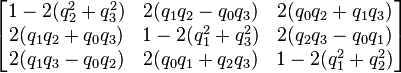
or equivalently, by the homogeneous expression:
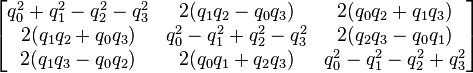
If  is not a unit quaternion then the homogeneous form is still a scalar multiple of a rotation matrix, while the inhomogeneous form is in general no longer an orthogonal matrix. This is why in numerical work the homogeneous form is to be preferred if distortion is to be avoided.
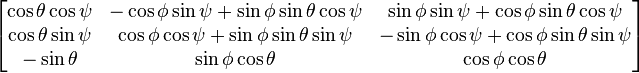
The direction cosine matrix (from the rotated Body XYZ coordinates to the original Lab xyz coordinates) corresponding to a Body 3-2-1 sequence with Euler angles (ψ, θ, φ) is given by:[1]
Conversion
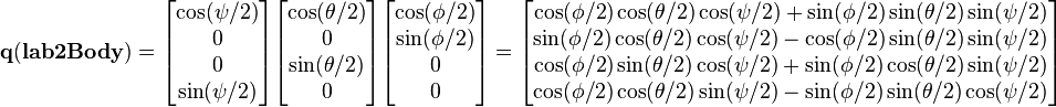
By combining the quaternion representations of the Euler rotations we get for the Body 3-2-1 sequence, where the airplane first does yaw (Body-Z) turn during taxiing on the runway, then pitches (Body-Y) during take-off, and finally rolls (Body-X) in the air. The resulting orientation of Body 3-2-1 sequence (around the capitalized axis in the illustration of Tait–Bryan angles) is equivalent to that of lab 1-2-3 sequence (around the lower-cased axis), where the airplane is rolled first (lab-x axis), and then nosed up around the horizontal lab-y axis, and finally rotated around the vertical lab-z axis:
Other rotation sequences use different conventions.[1]
For Euler angles we get:
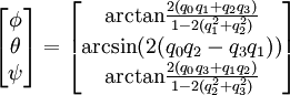
arctan and arcsin have a result between −π/2 and π/2. With three rotations between −π/2 and π/2 you can't have all possible orientations. We need to replace the arctan by atan2 to generate all the orientations.

Relationship with Tait–Bryan angles
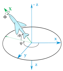
Similarly for Euler angles, we use the Tait–Bryan angles (in terms of flight dynamics):
- Roll –
 : rotation about the X-axis
 - Pitch –
 : rotation about the Y-axis
 - Yaw –
 : rotation about the Z-axis
where the X-axis points forward, Y-axis to the right and Z-axis downward and in the example to follow the rotation occurs in the order yaw, pitch, roll (about body-fixed axes).
Singularities
One must be aware of singularities in the Euler angle parametrization when the pitch approaches ±90° (north/south pole). These cases must be handled specially. The common name for this situation is gimbal lock.
Code to handle the singularities is derived on this site: www.euclideanspace.com
See also
- Rotation operator (vector space)
- Quaternions and spatial rotation
- Euler Angles
- Rotation matrix
- Rotation formalisms in three dimensions
References
- ↑ 1.0 1.1 NASA Mission Planning and Analysis Division. "Euler Angles, Quaternions, and Transformation Matrices" (PDF). NASA. Retrieved 12 January 2013.
External links
- Q60. How do I convert Euler rotation angles to a quaternion? and related questions at The Matrix and Quaternions FAQ