Controllability

Controllability is an important property of a control system, and the controllability property plays a crucial role in many control problems, such as stabilization of unstable systems by feedback, or optimal control.

Controllability and observability are dual aspects of the same problem.

Roughly, the concept of controllability denotes the ability to move a system around in its entire configuration space using only certain admissible manipulations. The exact definition varies slightly within the framework or the type of models applied.

The following are examples of variations of controllability notions which have been introduced in the systems and control literature:

State controllability
Output controllability
Controllability in the behavioural framework

State controllability

The state of a system, which is a collection of the system's variables values, completely describes the system at any given time. In particular, no information on the past of a system is needed to help in predicting the future, if the states at the present time are known.

Complete state controllability (or simply controllability if no other context is given) describes the ability of an external input to move the internal state of a system from any initial state to any other final state in a finite time interval.^[1]^:737

Continuous linear systems

Consider the continuous linear system ^{[note 1]}

\dot{\mathbf{x}}(t) = A(t) \mathbf{x}(t) + B(t) \mathbf{u}(t)

\mathbf{y}(t) = C(t) \mathbf{x}(t) + D(t) \mathbf{u}(t).

There exists a control $u$ from state $x_0$ at time $t_0$ to state $x_1$ at time $t_1 > t_0$ if and only if 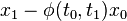$x_1 - \phi(t_0,t_1)x_0$ is in the column space of

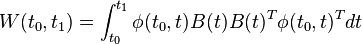
W(t_0,t_1) = \int_{t_0}^{t_1} \phi(t_0,t)B(t)B(t)^{T}\phi(t_0,t)^{T} dt

where $\phi$ is the state-transition matrix, and $W(t_0,t_1)$ is the Controllability Gramian.

In fact, if $\eta_0$ is a solution to $W(t_0,t_1)\eta = x_1 - \phi(t_0,t_1)x_0$ then a control given by 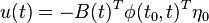$u(t) = -B(t)^{T}\phi(t_0,t)^{T}\eta_0$ would make the desired transfer.

Note that the matrix $W$ defined as above has the following properties:

$W(t_0,t_1)$ is symmetric
$W(t_0,t_1)$ is positive semidefinite for $t_1 \geq t_0$
$W(t_0,t_1)$ satisfies the linear matrix differential equation

\frac{d}{dt}W(t,t_1) = A(t)W(t,t_1)+W(t,t_1)A(t)^{T}-B(t)B(t)^{T}, \; W(t_1,t_1) = 0

$W(t_0,t_1)$ satisfies the equation

W(t_0,t_1) = W(t_0,t) + \phi(t_0,t)W(t,t_1)\phi(t_0,t)^{T}

^[2]

Continuous linear time-invariant (LTI) systems

Consider the continuous linear time-invariant system

\dot{\mathbf{x}}(t) = A \mathbf{x}(t) + B \mathbf{u}(t)

\mathbf{y}(t) = C \mathbf{x}(t) + D \mathbf{u}(t)

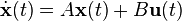
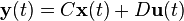
where

\mathbf{x}

is the

n \times 1

"state vector",

\mathbf{y}

is the

m \times 1

"output vector",

\mathbf{u}

is the

r \times 1

"input (or control) vector",

A

is the

n \times n

"state matrix",

B

is the

n \times r

"input matrix",

C

is the

m \times n

"output matrix",

D

is the

m \times r

"feedthrough (or feedforward) matrix".

The $n \times nr$ controllability matrix is given by

R = \begin{bmatrix}B & AB & A^{2}B & ...& A^{n-1}B\end{bmatrix}

The system is controllable if the controllability matrix has full row rank (i.e. 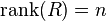$\operatorname{rank}(R)=n$ ).

Discrete linear time-invariant (LTI) systems

For a discrete-time linear state-space system (i.e. time variable $k\in\mathbb{Z}$ ) the state equation is

\textbf{x}(k+1) = A\textbf{x}(k) + B\textbf{u}(k)

Where $A$ is an $n \times n$ matrix and $B$ is a $n \times r$ matrix (i.e. $\mathbf{u}$ is $r$ inputs collected in a $r \times 1$ vector. The test for controllability is that the $n \times nr$ matrix

\mathcal{C} = \begin{bmatrix}B & AB & A^{2}B & \cdots & A^{n-1}B\end{bmatrix}

has full row rank (i.e., 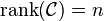$\operatorname{rank}(\mathcal C) = n$ ). That is, if the system is controllable, $\mathcal C$ will have $n$ columns that are linearly independent; if $n$ columns of $\mathcal C$ are linearly independent, each of the $n$ states is reachable giving the system proper inputs through the variable $u(k)$ .

Example

For example, consider the case when $n=2$ and $r=1$ (i.e. only one control input). Thus, $B$ and $A B$ are $2 \times 1$ vectors. If $\begin{bmatrix}B & AB\end{bmatrix}$ has rank 2 (full rank), and so $B$ and $AB$ are linearly independent and span the entire plane. If the rank is 1, then $B$ and $AB$ are collinear and do not span the plane.

Assume that the initial state is zero.

At time $k=0$ : $x(1) = A\textbf{x}(0) + B\textbf{u}(0) = B\textbf{u}(0)$

At time $k=1$ : $x(2) = A\textbf{x}(1) + B\textbf{u}(1) = AB\textbf{u}(0) + B\textbf{u}(1)$

At time $k=0$ all of the reachable states are on the line formed by the vector $B$ . At time $k=1$ all of the reachable states are linear combinations of $AB$ and $B$ . If the system is controllable then these two vectors can span the entire plane and can be done so for time $k=2$ . The assumption made that the initial state is zero is merely for convenience. Clearly if all states can be reached from the origin then any state can be reached from another state (merely a shift in coordinates).

This example holds for all positive $n$ , but the case of $n=2$ is easier to visualize.

Analogy for example of n = 2

Consider an analogy to the previous example system. You are sitting in your car on an infinite, flat plane and facing north. The goal is to reach any point in the plane by driving a distance in a straight line, come to a full stop, turn, and driving another distance, again, in a straight line. If your car has no steering then you can only drive straight, which means you can only drive on a line (in this case the north-south line since you started facing north). The lack of steering case would be analogous to when the rank of $C$ is 1 (the two distances you drove are on the same line).

Now, if your car did have steering then you could easily drive to any point in the plane and this would be the analogous case to when the rank of $C$ is 2.

If you change this example to $n=3$ then the analogy would be flying in space to reach any position in 3D space (ignoring the orientation of the aircraft). You are allowed to:

fly in a straight line
turn left or right by any amount (Yaw)
direct the plane upwards or downwards by any amount (Pitch)

Although the 3-dimensional case is harder to visualize, the concept of controllability is still analogous.

Nonlinear systems

Nonlinear systems in the control-affine form

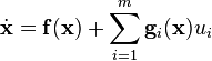
\dot{\mathbf{x}} = \mathbf{f(x)} + \sum_{i=1}^m \mathbf{g}_i(\mathbf{x})u_i

is locally accessible about $x_0$ if the accessibility distribution $R$ spans $n$ space, when $n$ equals the rank of $x$ and R is given by:^[3]

R = \begin{bmatrix} \mathbf{g}_1 & \cdots & \mathbf{g}_m & [\mathrm{ad}^k_{\mathbf{g}_i}\mathbf{\mathbf{g}_j}] & \cdots & [\mathrm{ad}^k_{\mathbf{f}}\mathbf{\mathbf{g}_i}] \end{bmatrix}.

Here, $[\mathrm{ad}^k_{\mathbf{f}}\mathbf{\mathbf{g}}]$ is the repeated Lie bracket operation defined by

[\mathrm{ad}^k_{\mathbf{f}}\mathbf{\mathbf{g}}] = \begin{bmatrix} \mathbf{f} & \cdots & j & \cdots & \mathbf{[\mathbf{f}, \mathbf{g}]} \end{bmatrix}.

The controllability matrix for linear systems in the previous section can in fact be derived from this equation.

Output controllability

Output controllability is the related notion for the output of the system; the output controllability describes the ability of an external input to move the output from any initial condition to any final condition in a finite time interval. It is not necessary that there is any relationship between state controllability and output controllability. In particular:

A controllable system is not necessarily output controllable. For example, if matrix D = 0 and matrix C does not have full row rank, then some positions of the output are masked by the limiting structure of the output matrix. Moreover, even though the system can be moved to any state in finite time, there may be some outputs that are inaccessible by all states. A trivial numerical example uses D=0 and a C matrix with at least one row of zeros; thus, the system is not able to produce a non-zero output along that dimension.
An output controllable system is not necessarily state controllable. For example, if the dimension of the state space is greater than the dimension of the output, then there will be a set of possible state configurations for each individual output. That is, the system can have significant zero dynamics, which are trajectories of the system that are not observable from the output. Consequently, being able to drive an output to a particular position in finite time says nothing about the state configuration of the system.

For a linear continuous-time system, like the example above, described by matrices $A$ , $B$ , $C$ , and $D$ , the $m \times (n+1)r$ output controllability matrix

\begin{bmatrix} CB & CAB & CA^2B & \cdots & CA^{n-1}B & D\end{bmatrix}

must have full row rank (i.e. rank $m$ ) if and only if the system is output controllable.^[1]^:742 This result is known as Kalman's criteria of controllability.

Controllability under input constraints

In systems with limited control authority, it is often no longer possible to move any initial state to any final state inside the controllable subspace. This phenomenon is caused by constraints on the input that could be inherent to the system (e.g. due to saturating actuator) or imposed on the system for other reasons (e.g. due to safety-related concerns). The controllability of systems with input and state constraints is studied in the context of reachability^[4] and viability theory.^[5]

Controllability in the behavioural framework

In the so-called behavioral system theoretic approach due to Willems (see people in systems and control), models considered do not directly define an input–output structure. In this framework systems are described by admissible trajectories of a collection of variables, some of which might be interpreted as inputs or outputs.

A system is then defined to be controllable in this setting, if any past part of a behavior (trajectory of the external veriables) can be concatenated with any future trajectory of the behavior in such a way that the concatenation is contained in the behavior, i.e. is part of the admissible system behavior.^[6]^:151

Stabilizability

A slightly weaker notion than controllability is that of stabilizability. A system is determined to be stabilizable when all uncontrollable states have stable dynamics. Thus, even though some of the states cannot be controlled (as determined by the controllability test above) all the states will still remain bounded during the system's behavior.^[7]

Notes

↑ A Linear time-invariant system behaves the same but with the coefficients are constant in time.

References

↑ 1.0 1.1 Katsuhiko Ogata (1997). Modern Control Engineering (3rd ed.). Upper Saddle River, NJ: Prentice-Hall. ISBN 0-13-227307-1.
↑ Brockett, Roger W. (1970). Finite Dimensional Linear Systems. John Wiley & Sons. ISBN 978-0-471-10585-5.
↑ Isidori, Alberto (1989). Nonlinear Control Systems, p. 92–3. Springer-Verlag, London. ISBN 3-540-19916-0.
↑ Claire J. Tomlin, Ian Mitchell, Alexandre M. Bayen and Meeko Oishi (2003). "Computational Techniques for the Verification of Hybrid Systems" (PDF). Proceedings of the IEEE. Retrieved 2012-03-04.
↑ Jean-Pierre Aubin (1991). Viability Theory. Birkhauser. ISBN 0-8176-3571-8.
↑ Jan Polderman, Jan Willems (1998). Introduction to Mathematical Systems Theory: A Behavioral Approach (1st ed.). New York: Springer Verlag. ISBN 0-387-98266-3.
↑ Brian D.O. Anderson; John B. Moore (1990). Optimal Control: Linear Quadratic Methods. Englewood Cliffs, NJ: Prentice Hall. ISBN 978-0-13-638560-8.

Controllability

State controllability

Continuous linear systems

Continuous linear time-invariant (LTI) systems

Discrete linear time-invariant (LTI) systems

Example

Analogy for example of n = 2

Nonlinear systems

Output controllability

Controllability under input constraints

Controllability in the behavioural framework

Stabilizability

See also

Notes

References

External links