Control-Lyapunov function
In control theory, a control-Lyapunov function[1] is a Lyapunov function  for a system with control inputs. The ordinary Lyapunov function is used to test whether a dynamical system is stable (more restrictively, asymptotically stable). That is, whether the system starting in a state
  in some domain D will remain in D, or for asymptotic stability will eventually return to
  . The control-Lyapunov function is used to test whether a system is feedback stabilizable, that is whether for any state x there exists a control
  such that the system can be brought to the zero state by applying the control u.
More formally, suppose we are given an autonomous dynamical system

where  is the state vector and
  is the control vector, and we want to feedback stabilize it to in some domain
  .
.
Definition. A control-Lyapunov function is a function  that is continuously differentiable, positive-definite (that is is positive except at where it is zero), and such that

The last condition is the key condition; in words it says that for each state x we can find a control u that will reduce the "energy" V. Intuitively, if in each state we can always find a way to reduce the energy, we should eventually be able to bring the energy to zero, that is to bring the system to a stop. This is made rigorous by the following result:
Artstein's theorem. The dynamical system has a differentiable control-Lyapunov function if and only if there exists a regular stabilizing feedback u(x).
It may not be easy to find a control-Lyapunov function for a given system, but if we can find one thanks to some ingenuity and luck, then the feedback stabilization problem simplifies considerably, in fact it reduces to solving a static non-linear programming problem

for each state x.
The theory and application of control-Lyapunov functions were developed by Z. Artstein and E. D. Sontag in the 1980s and 1990s.
Example
Here is a characteristic example of applying a Lyapunov candidate function to a control problem.
Consider the non-linear system, which is a mass-spring-damper system with spring hardening and position dependent mass described by

Now given the desired state,  , and actual state,
  , with error,
  , define a function
  as
as

A Control-Lyapunov candidate is then

which is positive definite for all  ,
,  .
.
Now taking the time derivative of 

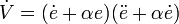
The goal is to get the time derivative to be

which is globally exponentially stable if is globally positive definite (which it is).
Hence we want the rightmost bracket of  ,
,
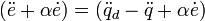
to fulfill the requirement
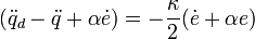
which upon substitution of the dynamics,  , gives
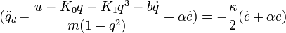
Solving for  yields the control law

with  and
and  , both greater than zero, as tunable parameters
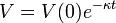
This control law will guarantee global exponential stability since upon substitution into the time derivative yields, as expected
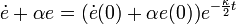
which is a linear first order differential equation which has solution
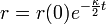
And hence the error and error rate, remembering that 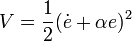 , exponentially decay to zero.
If you wish to tune a particular response from this, it is necessary to substitute back into the solution we derived for and solve for  . This is left as an exercise for the reader but the first few steps at the solution are:


which can then be solved using any linear differential equation methods.
Notes
- ↑ Freeman (46)
References
- Freeman, Randy A.; Petar V. Kokotović (2008). Robust Nonlinear Control Design (illustrated, reprint ed.). Birkhäuser. p. 257. ISBN 0-8176-4758-9. Retrieved 2009-03-04.