Consumption smoothing

Consumption smoothing is the economic concept used to express the desire of people to have a stable path of consumption. Since Milton Friedman's permanent income theory (1956) and Modigliani and Brumberg (1954) life-cycle model, the idea that agents prefer a stable path of consumption has been widely accepted.^[1]^[2] This idea came to replace the perception that people had a marginal propensity to consume and therefore current consumption was tied to current income.

Friedman's theory argues that consumption is linked to the permanent income of agents. Thus, when income is affected by transitory shocks, for example, agents' consumption should not change, since they can use savings or borrowing to adjust. This theory assumes that agents are able to finance consumption with earnings that are not yet generated, and thus assumes perfect capital markets. Empirical evidence shows that liquidity constraint is one of the main reasons why it is difficult to observe consumption smoothing in the data.

Model

Robert Hall (1978) formalized Friedman's idea.^[3] By taking into account the diminishing returns to consumption, and therefore, assuming a concave utility function, he showed that agents optimally would choose to keep a stable path of consumption.

With (cf. Hall's paper)

E_t

being the mathematical expectation conditional on all information available in

t

\delta = 1/\beta-1

being the agent's rate of time preference

r_t = R_t - 1\ge \delta

being the real rate of interest in

t

u

being the strictly concave one-period utility function

c_t

being the consumption in

t

y_t = w_t

being the earnings in

t

A_t

being the assets, apart from human capital, in

t

agents choose the consumption path that maximizes:

E_{0}\sum_{t=0}^{\infty }\beta^{t}\left[u(c_{t})\right]

Subject to a sequence of budget constraints:

A_{t+1}=R_{t+1}(A_{t}+y_{t}-c_{t})

The first order necessary condition in this case will be:

\beta E_{t}R_{t+1}\frac{u^{\prime }(c_{t+1})}{u^{\prime }(c_{t})}=1

By assuming that $R_{t+1}=R=\beta ^{-1}$ we obtain, for the previous equation:

E_{t}u^{\prime }(c_{t+1})=u^{\prime }(c_{t})

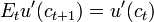
Which, due to the concavity of the utility function, implies:

E_{t}[c_{t+1}]=c_{t}

Thus, rational agents would expect to achieve the same consumption in every period.

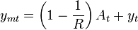
Hall also showed that for a quadratic utility function, the optimal consumption is equal to:

c_{t}=\left[ \frac{r}{1+r}\right] \left[ E_{t}\sum_{i=0}^{\infty }\left( \frac{1}{1+r}\right) ^{i}y_{t+i}+A_{t}\right]

This expression shows that agents choose to consume a fraction of their present discounted value of their human and financial wealth.

Criticism

Although Hall's proof, 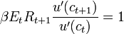$\beta E_{t}R_{t+1}\frac{u^{\prime }(c_{t+1})}{u^{\prime }(c_{t})}=1$ , is extremely short, just nine lines, Hall's corollary 4, $c_{t+1} = c_t$ , can be found in Flavin.^[4] Wu ^[5] has shown that changes in consumption being zero is the result of an error. Wu's proof is shown below applying the same definitions and techniques found in Sargent.^[6]

A consumer maximizes

\sum_{i=0}^{\infty} b^t \left[u_0+u_1c_1-\frac{u_2} {2} c_t ^2 \right],

subject to

A_t = R [A_t + y_t - c_t]

, where

y_t

, under a stochastic process, is

E_t y_t

where

c

is consumption,

A

is non-human assets,

y

is labor income,

R

is gross rate of return (all at the beginning of period).

E

is expectation,

t

is time.

Under the "Euler equation approach," optimal consumption for period t is given by

c_t=(1-R^{-2} b^{-1}) A_t - \frac{u_1}{u_2} \frac{(R^{-1} b^{-1} L^{-1})} {1 - R} + \frac{(1-R^{-2} b^{-1})} {1-L^{-1}R^{-1}} E_t y_t

, where,

L

is the lag operator

Repeating Euler optimization, one should find that consumption, $c_{t+1}, c_{t+2}, . . . , c_{t+n}$ , should be given by

c_{t+1}=(1-R^{-2} b^{-1}) A_{t+1} - \frac{u_1}{u_2} \frac{(R^{-1} b^{-1} L^{-1})} {1 - R} + \frac{(1-R^{-2} b^{-1})} {1-L^{-1}R^{-1}} E_{t+1} y_{t+1}

c_{t+2}=(1-R^{-2} b^{-1}) A_{t+2} - \frac{u_1}{u_2} \frac{(R^{-1} b^{-1} L^{-1})} {1 - R} + \frac{(1-R^{-2} b^{-1})} {1-L^{-1}R^{-1}} E_{t+2} y_{t+2}

. . .

c_{t+n}=(1-R^{-2} b^{-1}) A_{t+1} - \frac{u_1}{u_2} \frac{(R^{-1} b^{-1} L^{-1})} {1 - R} + \frac{(1-R^{-2} b^{-1})} {1-L^{-1}R^{-1}} E_{t+n} y_{t+n}

Assuming $Rb = 1$ ,

c_{t+n} = (1 - R^{-1}) \left[A_{t+n} + \frac{E_{t+n}y_{t+n}} {1-L^{-1}R^{-1}} \right]

Since $\frac{1} {1-RL}$ can be expanded as

\frac{1} {1-RL} = \frac{-(RL)^{-1}} {1-(RL)^{-1}} = -\frac{1} {R} L^{-1}- \left(\frac{1} {R} \right)^2 L^{-2} - \left(\frac{1} {R} \right) ^3 L^{-3} - . . .

and by definition of lag operator

L^{-n} y_t = y_{t+n}

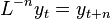
implies

\frac{(RL)^{-1}} {1-(RL)^{-1}} y_t = \frac{1} {R} L^{-1} y_{t} + \left(\frac{1} {R} \right)^2 L^{-2} y_{t} + \left(\frac{1} {R} \right) ^3 L^{-3} y_{t} + . . . = \sum_{j=1}^{\infty}\left( \frac{1}{R}\right) ^{j}y_{t+j}

thus for any n

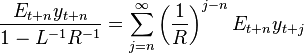
\frac{E_{t+n}y_{t+n}} {1-L^{-1}R^{-1}} = \sum_{j=n}^{\infty}\left( \frac{1}{R}\right) ^{j-n} E_{t+n} y_{t+j}

then

c_{t+n} = (1-R^{-1}) \left[A_{t+n} + \sum_{j=n}^{\infty}\left( \frac{1}{R}\right) ^{j-n} E_{t+n} y_{t+j} \right]

and for n = 1

c_{t+1} = (1-R^{-1}) \left[A_{t+1} + \sum_{j=1}^{\infty}\left( \frac{1}{R}\right) ^{j-1} E_{t+1} y_{t+j} \right]

Flavin's Mispecification

Flavin stated that

c_{t+1} = (1-R^{-1}) \left[A_{t+1} + \sum_{j=0}^{\infty}\left( \frac{1}{R}\right) ^{j} E_{t+1} y_{t+j+1} \right]

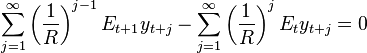
Flavin assumed that at period t+1, one still has the same number of incomes than at period t, i.e., sum of incomes from zero to infinity, instead of 1 to infinity. In fact, from one period to another, the number of income has to decline from n (where n tends to infinite) to n-1.

and found out that

c_{t+1} - c_t = (1-R^{-1}) \left[A_{t+1} -A_t + \sum_{j=0}^{\infty}\left( \frac{1}{R}\right) ^{j} E_{t+1} y_{t+j+1} - \sum_{j=0}^{\infty}\left( \frac{1}{R}\right) ^{j} E_{t} y_{t+j} \right] = (1-R^{-1}) \sum_{j=0}^{\infty}\left( \frac{1}{R}\right) ^{j} (E_{t+1} - E_{t}) y_{t+j+1}

and reached the Hall's conclusion that if the "expectations of future income are rational, the expectation of next period's revision in expectation, 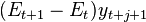$(E_{t+1} - E_{t}) y_{t+j+1}$ , is zero. Thus $E_t c_{t+1} = c_t$ ."

To see Flavin's mispecification, lets assume the case that $A_{t+1} - A_{t} = 0$ and that the 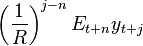$\left(\frac{1} {R}\right) ^{j-n} E_{t+n} {y_{t+j}}$ is $Y$ then

$c_t = A_{t} + n Y$ , where n tends to infinite and if one were to specify for $t+1$ that the sum varies from 1 to infinite, instead of 0 to infinite,

$c_{t+1} = A_{t+1} + (n-1) Y$ ,

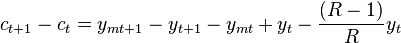
then the difference of consumption from one period to another is not zero but,

$c_{t+1} - c_{t} = - Y$

Restatement and Wu's Result

Applying the corrected $c_{t+1}$ , the change in consumption is,

c_{t+1} - c_t = (1-R^{-1}) \left[A_{t+1} -A_t + \sum_{j=1}^{\infty}\left( \frac{1}{R}\right) ^{j-1} E_{t+1} y_{t+j} - \sum_{j=0}^{\infty}\left( \frac{1}{R}\right) ^{j} E_{t} y_{t+j} \right]

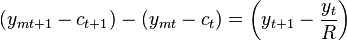
and since,

\sum_{j=0}^{\infty}\left( \frac{1}{R}\right) ^{j} E_{t} y_{t+j} = E_t y_t + \sum_{j=1}^{\infty}\left( \frac{1}{R}\right) ^{j} E_{t} y_{t+j} = y_t + \sum_{j=1}^{\infty}\left( \frac{1}{R}\right) ^{j} E_{t} y_{t+j}

If we assume that,

\sum_{j=1}^{\infty}\left( \frac{1}{R}\right) ^{j-1} E_{t+1} y_{t+j} - \sum_{j=1}^{\infty}\left( \frac{1}{R}\right) ^{j} E_{t} y_{t+j} = 0

and applying the definition of total income or "measured" income,

y_{mt} = \left(1- \frac{1} {R} \right) A_t + y_t

the change in consumption can be written as

c_{t+1} - c_t = y_{mt+1} - y_{t+1} - y_{mt} + y_t - \frac{(R-1)} {R} y_t

thus

change in savings =

(y_{mt+1} - c_{t+1}) - (y_{mt} - c_t) = \left( y_{t+1} - \frac{y_t} {R} \right)

Implications

Change in savings is a function of growth of labor income:

- any factor or policy affecting labor income growth will affect change in savings.

- income growth is dynamic leading to the disequilibrium model in Keynes ^[7] saving and disaving

- Clower's ^[8] dual decision hypothesis may help explain why unexpected changes in income makes consumers revise consumption and affect their change in savings

In practice, the relationship between change in savings and growth helps explain why:

- countries with rapid growth, e.g. those with trade surplus, have usually higher change in savings and countries with lower growth, e.g. trade deficit, lower change in saving. Net trade surplus countries such as Germany, China, Korea enjoy the highest gains in savings while countries such as U.S. loss in savings. Change in savings in Japan were high when trade was in surplus; now it is lower due to appreciation of Japanese Yen.

- depending on the intercept of savings vs growth, savings can turn negative even though growth is positive. Most economists, including Modigliani,^[9] have only considered growth vs savings, instead of change in savings. Case in point is the U.S. with positive growth and with saving rate bordering on negative.

- targeting a level of saving rate is meaningless, what matters is growth and change of savings.

Empirical Evidence

Robert Hall (1978) estimated the Euler equation in order to find evidence of a random walk in consumption. The data used are US National Income and Product Accounts (NIPA) quarterly from 1948 to 1977. For the analysis the author does not consider the consumption of durable goods. Although Hall argues that he finds some evidence of consumption smoothing, he does so using a modified version. There are also some econometric concerns about his findings.

Wilcox (1989) argue that liquidity constraint is the reason why consumption smoothing does not show up in the data.^[10] Zeldes (1989) follows the same argument and finds that a poor household's consumption is correlated with contemporaneous income, while a rich household's consumption is not.^[11]

References

↑ Friedman, Milton (1956). "A Theory of the Consumption Function." Princeton N. J.: Princeton University Press.
↑ Modigliani, F. & Brumberg, R. (1954): 'Utility analysis and the consumption function: An interpretation of cross-section data'. In: Kurihara, K.K (ed.): Post-Keynesian Economics
↑ Hall, Robert (1978). "Stochastic Implications of the Life Cycle-Permanent Income Hypothesis: Theory and Evidence." Journal of Political Economy, vol. 86, pp. 971-988.
↑ Flavin, M.A. (1977, published 1981), "The Adjustment of Consumption to Changing expectations about Future Income," Journal of Political Economy, vol. 89n, no. 5.
↑ Wu, C. K. (1996), "New Result in Theory of Consumption: Changes in Savings and Income Growth," https://ideas.repec.org/p/wpa/wuwpma/9706007.html
↑ Sargent, T. J. (1987), "Macroeconomic Theory," 2nd Edition, Academic Press.
↑ Keynes, J.M. (1936), "The General Theory of Employment, Interest, and Money," Hartcourt Brace Jovanovich.
↑ Clower, R.W. (1965), "The Keynesian Counterrevolution: A Theoretical Appraisal,", The Theory of Interest Rates, ed. F.H. Hahn and F.P.R. Brechling, Macmillan, p. 103-25.
↑ Modigliani, F. and Brumbert, R. (unpublished manuscript 1952, published 1979), "Utility Analysis and Aggregate Consumption Functions: An Attempt at Integration," Collected Papers of Franco Modigliani, ed. A. Abel, Vol. 2, MIT Press.
↑ Wilcox, James A. (1989). "Liquidity Constraints on Consumption: The Real Effects of Real Lending Policies." Federal Reserve Bank of San Francisco Economic Review, pp. 39-52.
↑ Zeldes, Stephen P. (1989). "Consumption and Liquidity Constraints: An Empirical Investigation." Journal of Political Economy, University of Chicago Press, vol. 97(2), pp. 305-46