Construction of t-norms

In mathematics, t-norms are a special kind of binary operations on the real unit interval [0, 1]. Various constructions of t-norms, either by explicit definition or by transformation from previously known functions, provide a plenitude of examples and classes of t-norms. This is important, e.g., for finding counter-examples or supplying t-norms with particular properties for use in engineering applications of fuzzy logic. The main ways of construction of t-norms include using generators, defining parametric classes of t-norms, rotations, or ordinal sums of t-norms.

Relevant background can be found in the article on t-norms.

Generators of t-norms

The method of constructing t-norms by generators consists in using a unary function (generator) to transform some known binary function (most often, addition or multiplication) into a t-norm.

In order to allow using non-bijective generators, which do not have the inverse function, the following notion of pseudo-inverse function is employed:

Let f: [a, b] → [c, d] be a monotone function between two closed subintervals of extended real line. The pseudo-inverse function to f is the function f ⁽⁻¹⁾: [c, d] → [a, b] defined as

f^{(-1)}(y) = \begin{cases} \sup \{ x\in[a,b] \mid f(x) < y \} & \text{for } f \text{ non-decreasing} \\ \sup \{ x\in[a,b] \mid f(x) > y \} & \text{for } f \text{ non-increasing.} \end{cases}

Additive generators

The construction of t-norms by additive generators is based on the following theorem:

Let f: [0, 1] → [0, +∞] be a strictly decreasing function such that f(1) = 0 and f(x) + f(y) is in the range of f or equal to f(0⁺) or +∞ for all x, y in [0, 1]. Then the function T: [0, 1]² → [0, 1] defined as

T(x, y) = f ^(-1)(f(x) + f(y))

is a t-norm.

If a t-norm T results from the latter construction by a function f which is right-continuous in 0, then f is called an additive generator of T.

Examples:

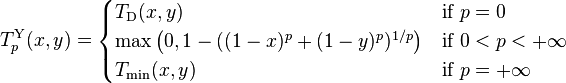
The function f(x) = 1 – x for x in [0, 1] is an additive generator of the Łukasiewicz t-norm.
The function f defined as f(x) = –log(x) if 0 < x ≤ 1 and f(0) = +∞ is an additive generator of the product t-norm.
The function f defined as f(x) = 2 – x if 0 ≤ x < 1 and f(1) = 0 is an additive generator of the drastic t-norm.

Basic properties of additive generators are summarized by the following theorem:

Let f: [0, 1] → [0, +∞] be an additive generator of a t-norm T. Then:

T is an Archimedean t-norm.
T is continuous if and only if f is continuous.
T is strictly monotone if and only if f(0) = +∞.
Each element of (0, 1) is a nilpotent element of T if and only if f(0) < +∞.
The multiple of f by a positive constant is also an additive generator of T.
T has no non-trivial idempotents. (Consequently, e.g., the minimum t-norm has no additive generator.)

Multiplicative generators

The isomorphism between addition on [0, +∞] and multiplication on [0, 1] by the logarithm and the exponential function allow two-way transformations between additive and multiplicative generators of a t-norm. If f is an additive generator of a t-norm T, then the function h: [0, 1] → [0, 1] defined as h(x) = e^−f (x) is a multiplicative generator of T, that is, a function h such that

h is strictly increasing
h(1) = 1
h(x) · h(y) is in the range of h or equal to 0 or h(0+) for all x, y in [0, 1]
h is right-continuous in 0
T(x, y) = h ⁽⁻¹⁾(h(x) · h(y)).

Vice versa, if h is a multiplicative generator of T, then f: [0, 1] → [0, +∞] defined by f(x) = −log(h(x)) is an additive generator of T.

Parametric classes of t-norms

Many families of related t-norms can be defined by an explicit formula depending on a parameter p. This section lists the best known parameterized families of t-norms. The following definitions will be used in the list:

A family of t-norms T_p parameterized by p is increasing if T_p(x, y) ≤ T_q(x, y) for all x, y in [0, 1] whenever p ≤ q (similarly for decreasing and strictly increasing or decreasing).

A family of t-norms T_p is continuous with respect to the parameter p if

\lim_{p\to p_0} T_p = T_{p_0}

for all values p₀ of the parameter.

Schweizer–Sklar t-norms

Graph (3D and contours) of the Schweizer–Sklar t-norm with p = 2

The family of Schweizer–Sklar t-norms, introduced by Berthold Schweizer and Abe Sklar in the early 1960s, is given by the parametric definition

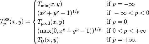
T^{\mathrm{SS}}_p(x,y) = \begin{cases} T_\min(x,y) & \text{if } p = -\infty \\ (x^p + y^p - 1)^{1/p} & \text{if } -\infty < p < 0 \\ T_{\mathrm{prod}}(x,y) & \text{if } p = 0 \\ (\max(0, x^p + y^p - 1))^{1/p} & \text{if } 0 < p < +\infty \\ T_{\mathrm{D}}(x,y) & \text{if } p = +\infty. \end{cases}

A Schweizer–Sklar t-norm $T^{\mathrm{SS}}_p$ is

Archimedean if and only if p > −∞
Continuous if and only if p < +∞
Strict if and only if −∞ < p ≤ 0 (for p = −1 it is the Hamacher product)
Nilpotent if and only if 0 < p < +∞ (for p = 1 it is the Łukasiewicz t-norm).

The family is strictly decreasing for p ≥ 0 and continuous with respect to p in [−∞, +∞]. An additive generator for $T^{\mathrm{SS}}_p$ for −∞ < p < +∞ is

f^{\mathrm{SS}}_p (x) = \begin{cases} -\log x & \text{if } p = 0 \\ \frac{1 - x^p}{p} & \text{otherwise.} \end{cases}

Hamacher t-norms

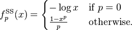
The family of Hamacher t-norms, introduced by Horst Hamacher in the late 1970s, is given by the following parametric definition for 0 ≤ p ≤ +∞:

T^{\mathrm{H}}_p (x,y) = \begin{cases} T_{\mathrm{D}}(x,y) & \text{if } p = +\infty \\ 0 & \text{if } p = x = y = 0 \\ \frac{xy}{p + (1 - p)(x + y - xy)} & \text{otherwise.} \end{cases}

The t-norm $T^{\mathrm{H}}_0$ is called the Hamacher product.

Hamacher t-norms are the only t-norms which are rational functions. The Hamacher t-norm $T^{\mathrm{H}}_p$ is strict if and only if p < +∞ (for p = 1 it is the product t-norm). The family is strictly decreasing and continuous with respect to p. An additive generator of $T^{\mathrm{H}}_p$ for p < +∞ is

f^{\mathrm{H}}_p(x) = \begin{cases} \frac{1 - x}{x} & \text{if } p = 0 \\ \log\frac{p + (1 - p)x}{x} & \text{otherwise.} \end{cases}

Frank t-norms

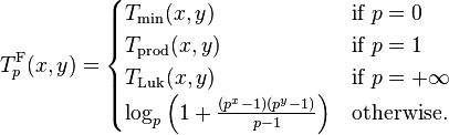
The family of Frank t-norms, introduced by M.J. Frank in the late 1970s, is given by the parametric definition for 0 ≤ p ≤ +∞ as follows:

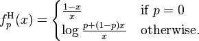
T^{\mathrm{F}}_p(x,y) = \begin{cases} T_{\mathrm{min}}(x,y) & \text{if } p = 0 \\ T_{\mathrm{prod}}(x,y) & \text{if } p = 1 \\ T_{\mathrm{Luk}}(x,y) & \text{if } p = +\infty \\ \log_p\left(1 + \frac{(p^x - 1)(p^y - 1)}{p - 1}\right) & \text{otherwise.} \end{cases}

The Frank t-norm $T^{\mathrm{F}}_p$ is strict if p < +∞. The family is strictly decreasing and continuous with respect to p. An additive generator for $T^{\mathrm{F}}_p$ is

f^{\mathrm{F}}_p(x) = \begin{cases} -\log x & \text{if } p = 1 \\ 1 - x & \text{if } p = +\infty \\ \log\frac{p - 1}{p^x - 1} & \text{otherwise.} \end{cases}

Yager t-norms

Graph of the Yager t-norm with p = 2

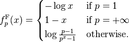
The family of Yager t-norms, introduced in the early 1980s by Ronald R. Yager, is given for 0 ≤ p ≤ +∞ by

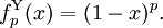
T^{\mathrm{Y}}_p (x,y) = \begin{cases} T_{\mathrm{D}}(x,y) & \text{if } p = 0 \\ \max\left(0, 1 - ((1 - x)^p + (1 - y)^p)^{1/p}\right) & \text{if } 0 < p < +\infty \\ T_{\mathrm{min}}(x,y) & \text{if } p = +\infty \end{cases}

The Yager t-norm $T^{\mathrm{Y}}_p$ is nilpotent if and only if 0 < p < +∞ (for p = 1 it is the Łukasiewicz t-norm). The family is strictly increasing and continuous with respect to p. The Yager t-norm $T^{\mathrm{Y}}_p$ for 0 < p < +∞ arises from the Łukasiewicz t-norm by raising its additive generator to the power of p. An additive generator of $T^{\mathrm{Y}}_p$ for 0 < p < +∞ is

f^{\mathrm{Y}}_p(x) = (1 - x)^p.

Aczél–Alsina t-norms

The family of Aczél–Alsina t-norms, introduced in the early 1980s by János Aczél and Claudi Alsina, is given for 0 ≤ p ≤ +∞ by

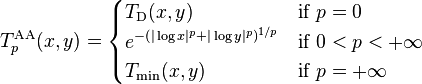
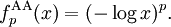
T^{\mathrm{AA}}_p (x,y) = \begin{cases} T_{\mathrm{D}}(x,y) & \text{if } p = 0 \\ e^{-\left(|\log x|^p + |\log y|^p\right)^{1/p}} & \text{if } 0 < p < +\infty \\ T_{\mathrm{min}}(x,y) & \text{if } p = +\infty \end{cases}

The Aczél–Alsina t-norm $T^{\mathrm{AA}}_p$ is strict if and only if 0 < p < +∞ (for p = 1 it is the product t-norm). The family is strictly increasing and continuous with respect to p. The Aczél–Alsina t-norm $T^{\mathrm{AA}}_p$ for 0 < p < +∞ arises from the product t-norm by raising its additive generator to the power of p. An additive generator of $T^{\mathrm{AA}}_p$ for 0 < p < +∞ is

f^{\mathrm{AA}}_p(x) = (-\log x)^p.

Dombi t-norms

The family of Dombi t-norms, introduced by József Dombi (1982), is given for 0 ≤ p ≤ +∞ by

T^{\mathrm{D}}_p (x,y) = \begin{cases} 0 & \text{if } x = 0 \text{ or } y = 0 \\ T_{\mathrm{D}}(x,y) & \text{if } p = 0 \\ T_{\mathrm{min}}(x,y) & \text{if } p = +\infty \\ \frac{1}{1 + \left( \left(\frac{1 - x}{x}\right)^p + \left(\frac{1 - y}{y}\right)^p \right)^{1/p}} & \text{otherwise.} \\ \end{cases}

The Dombi t-norm $T^{\mathrm{D}}_p$ is strict if and only if 0 < p < +∞ (for p = 1 it is the Hamacher product). The family is strictly increasing and continuous with respect to p. The Dombi t-norm $T^{\mathrm{D}}_p$ for 0 < p < +∞ arises from the Hamacher product t-norm by raising its additive generator to the power of p. An additive generator of $T^{\mathrm{D}}_p$ for 0 < p < +∞ is

f^{\mathrm{D}}_p(x) = \left(\frac{1-x}{x}\right)^p.

Sugeno–Weber t-norms

The family of Sugeno–Weber t-norms was introduced in the early 1980s by Siegfried Weber; the dual t-conorms were defined already in the early 1970s by Michio Sugeno. It is given for −1 ≤ p ≤ +∞ by

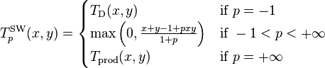
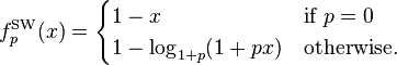
T^{\mathrm{SW}}_p (x,y) = \begin{cases} T_{\mathrm{D}}(x,y) & \text{if } p = -1 \\ \max\left(0, \frac{x + y - 1 + pxy}{1 + p}\right) & \text{if } -1 < p < +\infty \\ T_{\mathrm{prod}}(x,y) & \text{if } p = +\infty \end{cases}

The Sugeno–Weber t-norm $T^{\mathrm{SW}}_p$ is nilpotent if and only if −1 < p < +∞ (for p = 0 it is the Łukasiewicz t-norm). The family is strictly increasing and continuous with respect to p. An additive generator of $T^{\mathrm{SW}}_p$ for 0 < p < +∞ [sic] is

f^{\mathrm{SW}}_p(x) = \begin{cases} 1 - x & \text{if } p = 0 \\ 1 - \log_{1 + p}(1 + px) & \text{otherwise.} \end{cases}

Ordinal sums

The ordinal sum constructs a t-norm from a family of t-norms, by shrinking them into disjoint subintervals of the interval [0, 1] and completing the t-norm by using the minimum on the rest of the unit square. It is based on the following theorem:

Let T_i for i in an index set I be a family of t-norms and (a_i, b_i) a family of pairwise disjoint (non-empty) open subintervals of [0, 1]. Then the function T: [0, 1]² → [0, 1] defined as

T(x, y) = \begin{cases} a_i + (b_i - a_i) \cdot T_i\left(\frac{x - a_i}{b_i - a_i}, \frac{y - a_i}{b_i - a_i}\right) & \text{if } x, y \in [a_i, b_i]^2 \\ \min(x, y) & \text{otherwise} \end{cases}

is a t-norm.

Ordinal sum of the Łukasiewicz t-norm on the interval [0.05, 0.45] and the product t-norm on the interval [0.55, 0.95]

The resulting t-norm is called the ordinal sum of the summands (T_i, a_i, b_i) for i in I, denoted by

T = \bigoplus\nolimits_{i\in I} (T_i, a_i, b_i),

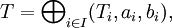
or $(T_1, a_1, b_1) \oplus \dots \oplus (T_n, a_n, b_n)$ if I is finite.

Ordinal sums of t-norms enjoy the following properties:

Each t-norm is a trivial ordinal sum of itself on the whole interval [0, 1].

The empty ordinal sum (for the empty index set) yields the minimum t-norm T_min. Summands with the minimum t-norm can arbitrarily be added or omitted without changing the resulting t-norm.

It can be assumed without loss of generality that the index set is countable, since the real line can only contain at most countably many disjoint subintervals.

An ordinal sum of t-norm is continuous if and only if each summand is a continuous t-norm. (Analogously for left-continuity.)

An ordinal sum is Archimedean if and only if it is a trivial sum of one Archimedean t-norm on the whole unit interval.

An ordinal sum has zero divisors if and only if for some index i, a_i = 0 and T_i has zero divisors. (Analogously for nilpotent elements.)

If 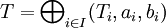$T = \bigoplus\nolimits_{i\in I} (T_i, a_i, b_i)$ is a left-continuous t-norm, then its residuum R is given as follows:

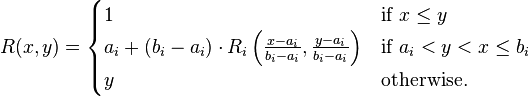
R(x, y) = \begin{cases} 1 & \text{if } x \le y \\ a_i + (b_i - a_i) \cdot R_i\left(\frac{x - a_i}{b_i - a_i}, \frac{y - a_i}{b_i - a_i}\right) & \text{if } a_i < y < x \le b_i \\ y & \text{otherwise.} \end{cases}

where R_i is the residuum of T_i, for each i in I.

Ordinal sums of continuous t-norms

The ordinal sum of a family of continuous t-norms is a continuous t-norm. By the Mostert–Shields theorem, every continuous t-norm is expressible as the ordinal sum of Archimedean continuous t-norms. Since the latter are either nilpotent (and then isomorphic to the Łukasiewicz t-norm) or strict (then isomorphic to the product t-norm), each continuous t-norm is isomorphic to the ordinal sum of Łukasiewicz and product t-norms.

Important examples of ordinal sums of continuous t-norms are the following ones:

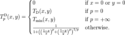
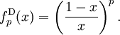
Dubois–Prade t-norms, introduced by Didier Dubois and Henri Prade in the early 1980s, are the ordinal sums of the product t-norm on [0, p] for a parameter p in [0, 1] and the (default) minimum t-norm on the rest of the unit interval. The family of Dubois–Prade t-norms is decreasing and continuous with respect to p..

Mayor–Torrens t-norms, introduced by Gaspar Mayor and Joan Torrens in the early 1990s, are the ordinal sums of the Łukasiewicz t-norm on [0, p] for a parameter p in [0, 1] and the (default) minimum t-norm on the rest of the unit interval. The family of Mayor–Torrens t-norms is decreasing and continuous with respect to p..

Rotations

The construction of t-norms by rotation was introduced by Sándor Jenei (2000). It is based on the following theorem:

Let T be a left-continuous t-norm without zero divisors, N: [0, 1] → [0, 1] the function that assigns 1 − x to x and t = 0.5. Let T₁ be the linear transformation of T into [t, 1] and

R_{T_1}(x,y) = \sup\{z \mid T_1(z,x)\le y\}.

Then the function

T_{\mathrm{rot}} = \begin{cases} T_1(x, y) & \text{if } x, y \in (t, 1] \\ N(R_{T_1}(x, N(y))) & \text{if } x \in (t, 1] \text{ and } y \in [0, t] \\ N(R_{T_1}(y, N(x))) & \text{if } x \in [0, t] \text{ and } y \in (t, 1] \\ 0 & \text{if } x, y \in [0, t] \end{cases}

is a left-continuous t-norm, called the rotation of the t-norm T.

The nilpotent minimum as a rotation of the minimum t-norm

Geometrically, the construction can be described as first shrinking the t-norm T to the interval [0.5, 1] and then rotating it by the angle 2π/3 in both directions around the line connecting the points (0, 0, 1) and (1, 1, 0).

Rotations of the Łukasiewicz, product, nilpotent minimum, and drastic t-norm

The theorem can be generalized by taking for N any strong negation, that is, an involutive strictly decreasing continuous function on [0, 1], and for t taking the unique fixed point of N.

The resulting t-norm enjoys the following rotation invariance property with respect to N:

T(x, y) ≤ z if and only if T(y, N(z)) ≤ N(x) for all x, y, z in [0, 1].

The negation induced by T_rot is the function N, that is, N(x) = R_rot(x, 0) for all x, where R_rot is the residuum of T_rot.

References

Klement, Erich Peter; Mesiar, Radko; and Pap, Endre (2000), Triangular Norms. Dordrecht: Kluwer. ISBN 0-7923-6416-3.
Fodor, János (2004), "Left-continuous t-norms in fuzzy logic: An overview". Acta Polytechnica Hungarica 1(2), ISSN 1785-8860
Dombi, József (1982), "A general class of fuzzy operators, the DeMorgan class of fuzzy operators and fuzziness measures induced by fuzzy operators". Fuzzy Sets and Systems 8, 149–163.
Jenei, Sándor (2000), "Structure of left-continuous t-norms with strong induced negations. (I) Rotation construction". Journal of Applied Non-Classical Logics 10, 83–92.
Mirko Navara (2007), "Triangular norms and conorms", Scholarpedia .