Conditional independence

Probability theory

Probability axioms
Probability space Sample space Elementary event Event Random variable Probability measure
Complementary event Joint probability Marginal probability Conditional probability
Independence Conditional independence Law of total probability Law of large numbers Bayes' theorem Boole's inequality
Venn diagram Tree diagram

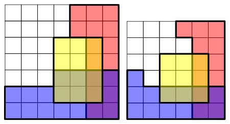
In probability theory, two events R and B are conditionally independent given a third event Y precisely if the occurrence or non-occurrence of R and the occurrence or non-occurrence of B are independent events in their conditional probability distribution given Y. In other words, R and B are conditionally independent given Y if and only if, given knowledge that Y occurs, knowledge of whether R occurs provides no information on the likelihood of B occurring, and knowledge of whether B occurs provides no information on the likelihood of R occurring.

Formal definition

These are two examples illustrating conditional independence. Each cell represents a possible outcome. The events R, B and Y are represented by the areas shaded red, blue and yellow respectively. And the probabilities of these events are shaded areas with respect to the total area. In both examples R and B are conditionally independent given Y because:

\Pr(R \cap B \mid Y) = \Pr(R \mid Y)\Pr(B \mid Y)\,

^[1]
but not conditionally independent given not Y because: :

\Pr(R \cap B \mid \text{not } Y) \not= \Pr(R \mid \text{not } Y)\Pr(B \mid \text{not } Y).\,

In the standard notation of probability theory, R and B are conditionally independent given Y if and only if

\Pr(R \cap B \mid Y) = \Pr(R \mid Y)\Pr(B \mid Y),\,

or equivalently,

\Pr(R \mid B \cap Y) = \Pr(R \mid Y).\,

Two random variables X and Y are conditionally independent given a third random variable Z if and only if they are independent in their conditional probability distribution given Z. That is, X and Y are conditionally independent given Z if and only if, given any value of Z, the probability distribution of X is the same for all values of Y and the probability distribution of Y is the same for all values of X.

Two events R and B are conditionally independent given a σ-algebra Σ if

\Pr(R \cap B \mid \Sigma) = \Pr(R \mid \Sigma)\Pr(B \mid \Sigma)\ a.s.

where $\Pr(A \mid \Sigma)$ denotes the conditional expectation of the indicator function of the event $A$ , $\chi_A$ , given the sigma algebra $\Sigma$ . That is,

\Pr(A \mid \Sigma) := \operatorname{E}[\chi_A\mid\Sigma].

Two random variables X and Y are conditionally independent given a σ-algebra Σ if the above equation holds for all R in σ(X) and B in σ(Y).

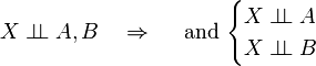
Two random variables X and Y are conditionally independent given a random variable W if they are independent given σ(W): the σ-algebra generated by W. This is commonly written:

X \perp\!\!\!\perp Y \mid W

X \perp Y \mid W

This is read "X is independent of Y, given W"; the conditioning applies to the whole statement: "(X is independent of Y) given W".

(X \perp\!\!\!\perp Y) \mid W

If W assumes a countable set of values, this is equivalent to the conditional independence of X and Y for the events of the form [W = w]. Conditional independence of more than two events, or of more than two random variables, is defined analogously.

The following two examples show that X ⊥ Y neither implies nor is implied by X ⊥ Y | W. First, suppose W is 0 with probability 0.5 and is the value 1 otherwise. When W = 0 take X and Y to be independent, each having the value 0 with probability 0.99 and the value 1 otherwise. When W = 1, X and Y are again independent, but this time they take the value 1 with probability 0.99. Then X ⊥ Y | W. But X and Y are dependent, because Pr(X = 0) < Pr(X = 0|Y = 0). This is because Pr(X = 0) = 0.5, but if Y = 0 then it's very likely that W = 0 and thus that X = 0 as well, so Pr(X = 0|Y = 0) > 0.5. For the second example, suppose X ⊥ Y, each taking the values 0 and 1 with probability 0.5. Let W be the product X×Y. Then when W = 0, Pr(X = 0) = 2/3, but Pr(X = 0|Y = 0) = 1/2, so X ⊥ Y | W is false. This is also an example of Explaining Away. See Kevin Murphy's tutorial ^[2] where X and Y take the values "brainy" and "sporty".

Uses in Bayesian inference

Let p be the proportion of voters who will vote "yes" in an upcoming referendum. In taking an opinion poll, one chooses n voters randomly from the population. For i = 1, ..., n, let X_i = 1 or 0 according as the ith chosen voter will or will not vote "yes".

In a frequentist approach to statistical inference one would not attribute any probability distribution to p (unless the probabilities could be somehow interpreted as relative frequencies of occurrence of some event or as proportions of some population) and one would say that X₁, ..., X_n are independent random variables.

By contrast, in a Bayesian approach to statistical inference, one would assign a probability distribution to p regardless of the non-existence of any such "frequency" interpretation, and one would construe the probabilities as degrees of belief that p is in any interval to which a probability is assigned. In that model, the random variables X₁, ..., X_n are not independent, but they are conditionally independent given the value of p. In particular, if a large number of the Xs are observed to be equal to 1, that would imply a high conditional probability, given that observation, that p is near 1, and thus a high conditional probability, given that observation, that the next X to be observed will be equal to 1.

Rules of conditional independence

A set of rules governing statements of conditional independence have been derived from the basic definition.^[3]^[4]

Note: since these implications hold for any probability space, they will still hold if one considers a sub-universe by conditioning everything on another variable, say K. For example, $X \perp\!\!\!\perp Y \Rightarrow Y \perp\!\!\!\perp X$ would also mean that $X \perp\!\!\!\perp Y \mid K \Rightarrow Y \perp\!\!\!\perp X \mid K$ .

Note: below, the comma can be read as an "AND".

Symmetry

X \perp\!\!\!\perp Y \quad \Rightarrow \quad Y \perp\!\!\!\perp X

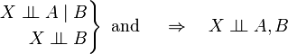
Decomposition

X \perp\!\!\!\perp A,B \quad \Rightarrow \quad \text{ and } \begin{cases} X \perp\!\!\!\perp A \\ X \perp\!\!\!\perp B \end{cases}

Proof:

$p_{X,A,B}(x,a,b) = p_X(x) p_{A,B}(a,b)$ (meaning of $X \perp A,B$ )
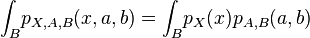$\int_{B} \! p_{X,A,B}(x,a,b) = \int_{B} \! p_X(x) p_{A,B}(a,b)$ (ignore variable B by integrating it out)
$p_{X,A}(x,a) = p_X(x) p_A(a)$

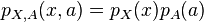
A similar proof shows the independence of X and B.

Weak union

X \perp\!\!\!\perp A,B \quad \Rightarrow \quad X \perp\!\!\!\perp A \mid B

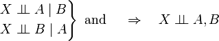
Contraction

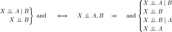
\left.\begin{align} X \perp\!\!\!\perp A \mid B \\ X \perp\!\!\!\perp B \end{align}\right\}\text{ and } \quad \Rightarrow \quad X \perp\!\!\!\perp A,B

Contraction-weak-union-decomposition

Putting the above three together, we have:

\left.\begin{align} X \perp\!\!\!\perp A \mid B \\ X \perp\!\!\!\perp B \end{align}\right\}\text{ and } \quad \iff \quad X \perp\!\!\!\perp A,B \quad \Rightarrow \quad \text{ and } \begin{cases} X \perp\!\!\!\perp A \mid B \\ X \perp\!\!\!\perp B \\ X \perp\!\!\!\perp B \mid A \\ X \perp\!\!\!\perp A \\ \end{cases}

Intersection

If the probabilities of X, A, B are all positive, then the following also holds:

\left.\begin{align} X \perp\!\!\!\perp A \mid B \\ X \perp\!\!\!\perp B \mid A \end{align}\right\}\text{ and } \quad \Rightarrow \quad X \perp\!\!\!\perp A, B

The five rules above were termed "Graphoid Axioms" by Pearl and Paz,^[5] because they hold in graphs, if $X \perp\!\!\!\perp A\mid B$ is interpreted to mean: "All paths from X to A are intercepted by the set B".^[6]

References

↑ To see that this is the case, one needs to realise that Pr(R ∩ B | Y) is the probability of an overlap of R and B (the purple shaded area) in the Y area. Since, in the picture on the left, there are two squares where R and B overlap within the Y area, and the Y area has twelve squares, Pr(R ∩ B | Y) = 2/12 = 1/6. Similarly, Pr(R | Y) = 4/12 = 1/3 and Pr(B | Y) = 6/12 = 1/2.
↑ http://people.cs.ubc.ca/~murphyk/Bayes/bnintro.html
↑ Dawid, A. P. (1979). "Conditional Independence in Statistical Theory". Journal of the Royal Statistical Society, Series B 41 (1): 1–31. JSTOR 2984718. MR 0535541.
↑ J Pearl, Causality: Models, Reasoning, and Inference, 2000, Cambridge University Press
↑ Pearl, Judea; Paz, Azaria (1985). "Graphoids: A Graph-Based Logic for Reasoning About Relevance Relations". Missing or empty |url= (help)
↑ Pearl, Judea (1988). Probabilistic reasoning in intelligent systems: networks of plausible inference. Morgan Kaufmann.