Column space
In linear algebra, the column space C(A) of a matrix A (sometimes called the range of a matrix) is the set of all possible linear combinations of its column vectors.
Let K be a field (such as real or complex numbers). The column space of an m × n matrix with components from K is a linear subspace of the m-space Km. The dimension of the column space is called the rank of the matrix.[1] A definition for matrices over a ring K (such as integers) is also possible.
The column space of a matrix is the image or range of the corresponding matrix transformation.
Definition
Let K be a field of scalars. Let A be an m × n matrix, with column vectors v1, v2, ..., vn. A linear combination of these vectors is any vector of the form

where c1, c2, ..., cn are scalars. The set of all possible linear combinations of v1, ... ,vn is called the column space of A. That is, the column space of A is the span of the vectors v1, ... , vn.
Any linear combination of the column vectors of a matrix A can be written as the product of A with a column vector:
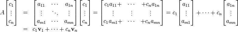
Therefore, the column space of A consists of all possible products Ax, for x ∈ Cn. This is the same as the image (or range) of the corresponding matrix transformation.
- Example
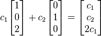
- If
 , then the column vectors are v1 = (1, 0, 2)T and v2 = (0, 1, 0)T.
 - A linear combination of v1 and v2 is any vector of the form
- The set of all such vectors is the column space of A. In this case, the column space is precisely the set of vectors (x, y, z) ∈ R3 satisfying the equation z = 2x (using Cartesian coordinates, this set is a plane through the origin in three-dimensional space).
Basis
The columns of A span the column space, but they may not form a basis if the column vectors are not linearly independent. Fortunately, elementary row operations do not affect the dependence relations between the column vectors. This makes it possible to use row reduction to find a basis for the column space.
For example, consider the matrix
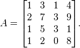
The columns of this matrix span the column space, but they may not be linearly independent, in which case some subset of them will form a basis. To find this basis, we reduce A to reduced row echelon form:
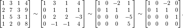
At this point, it is clear that the first, second, and fourth columns are linearly independent, while the third column is a linear combination of the first two. (Specifically, v3 = –2v1 + v2.) Therefore, the first, second, and fourth columns of the original matrix are a basis for the column space:

Note that the independent columns of the reduced row echelon form are precisely the columns with pivots. This makes it possible to determine which columns are linearly independent by reducing only to echelon form.
The above algorithm can be used in general to find the dependence relations between any set of vectors, and to pick out a basis from any spanning set. A different algorithm for finding a basis from a spanning set is given in the row space article; finding a basis for the column space of A is equivalent to finding a basis for the row space of the transpose matrix AT.
Dimension
The dimension of the column space is called the rank of the matrix. The rank is equal to the number of pivots in the reduced row echelon form, and is the maximum number of linearly independent columns that can be chosen from the matrix. For example, the 4 × 4 matrix in the example above has rank three.
Because the column space is the image of the corresponding matrix transformation, the rank of a matrix is the same as the dimension of the image. For example, the transformation R4 → R4 described by the matrix above maps all of R4 to some four-dimensional subspace.
The nullity of a matrix is the dimension of the null space, and is equal to the number of columns in the reduced row echelon form that do not have pivots.[3] The rank and nullity of a matrix A with n columns are related by the equation:

This is known as the rank-nullity theorem.
Relation to the left null space
The left null space of A is the set of all vectors x such that xTA = 0T. It is the same as the null space of the transpose of A. The product of the matrix AT and the vector x can be written in terms of the dot product of vectors:
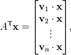
because row vectors of AT are transposes of column vectors vk of A. Thus ATx = 0 if and only if x is orthogonal (perpendicular) to each of the column vectors of A.
It follows that the left null space (the null space of AT) is the orthogonal complement to the column space of A.
For a matrix A, the column space, row space, null space, and left null space are sometimes referred to as the four fundamental subspaces.
For matrices over a ring
Similarly the column space (sometimes disambiguated as right column space) can be defined for matrices over a ring K as

for any c1, ..., cn, with replacement of the vector m-space with "right free module", which changes the order of scalar multiplication of the vector vk to the scalar ck such that it is written in an unusual order vector–scalar.[4]
See also
- Euclidean subspace
- Kernel (matrix)
- Row space
- Four fundamental subspaces
- Rank (linear algebra)
- Linear span
- Matrix (mathematics)
Notes
- ↑ Linear algebra, as discussed in this article, is a very well established mathematical discipline for which there are many sources. Almost all of the material in this article can be found in Lay 2005, Meyer 2001, and Strang 2005.
- ↑ This computation uses the Gauss–Jordan row-reduction algorithm. Each of the shown steps involves multiple elementary row operations.
- ↑ Columns without pivots represent free variables in the associated homogeneous system of linear equations.
- ↑ Important only if K is not commutative. Actually, this form is merely a product Ac of the matrix A to the column vector c from Kn where the order of factors is preserved, unlike the formula above.
References
Textbooks
- Strang, Gilbert (July 19, 2005), Linear Algebra and Its Applications (4th ed.), Brooks Cole, ISBN 978-0-03-010567-8
- Axler, Sheldon Jay (1997), Linear Algebra Done Right (2nd ed.), Springer-Verlag, ISBN 0-387-98259-0
- Lay, David C. (August 22, 2005), Linear Algebra and Its Applications (3rd ed.), Addison Wesley, ISBN 978-0-321-28713-7
- Meyer, Carl D. (February 15, 2001), Matrix Analysis and Applied Linear Algebra, Society for Industrial and Applied Mathematics (SIAM), ISBN 978-0-89871-454-8
- Poole, David (2006), Linear Algebra: A Modern Introduction (2nd ed.), Brooks/Cole, ISBN 0-534-99845-3
- Anton, Howard (2005), Elementary Linear Algebra (Applications Version) (9th ed.), Wiley International
- Leon, Steven J. (2006), Linear Algebra With Applications (7th ed.), Pearson Prentice Hall
External links
| Wikibooks has a book on the topic of: Linear Algebra/Column and Row Spaces |
- Khan Academy video tutorial
- Weisstein, Eric W., "Column Space", MathWorld.
- Gilbert Strang, MIT Linear Algebra Lecture on the Four Fundamental Subspaces at Google Video, from MIT OpenCourseWare