Cohen's kappa
Cohen's kappa coefficient is a statistic which measures inter-rater agreement for qualitative (categorical) items. It is generally thought to be a more robust measure than simple percent agreement calculation, since κ takes into account the agreement occurring by chance. [1] Some researchers[2] have expressed concern over κ's tendency to take the observed categories' frequencies as givens, which can have the effect of underestimating agreement for a category that is also commonly used; for this reason, κ is considered an overly conservative measure of agreement. Others[3] contest the assertion that kappa "takes into account" chance agreement. To do this effectively would require an explicit model of how chance affects rater decisions. The so-called chance adjustment of kappa statistics supposes that, when not completely certain, raters simply guess—a very unrealistic scenario.
Calculation
Cohen's kappa measures the agreement between two raters who each classify N items into C mutually exclusive categories. The first mention of a kappa-like statistic is attributed to Galton (1892),[4] see Smeeton (1985).[5]
The equation for κ is:
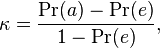
where Pr(a) is the relative observed agreement among raters, and Pr(e) is the hypothetical probability of chance agreement, using the observed data to calculate the probabilities of each observer randomly saying each category. If the raters are in complete agreement then κ = 1. If there is no agreement among the raters other than what would be expected by chance (as defined by Pr(e)), κ = 0.
The seminal paper introducing kappa as a new technique was published by Jacob Cohen in the journal Educational and Psychological Measurement in 1960.[6]
A similar statistic, called pi, was proposed by Scott (1955). Cohen's kappa and Scott's pi differ in terms of how Pr(e) is calculated.
Note that Cohen's kappa measures agreement between two raters only. For a similar measure of agreement (Fleiss' kappa) used when there are more than two raters, see Fleiss (1971). The Fleiss kappa, however, is a multi-rater generalization of Scott's pi statistic, not Cohen's kappa. Kappa is also used to compare performance in Machine Learning but the directional version known as Informedness or Youden's J statistic is argued to be more appropriate for supervised learning.[7]
Example
Suppose that you were analyzing data related to a group of 50 people applying for a grant. Each grant proposal was read by two readers and each reader either said "Yes" or "No" to the proposal. Suppose the dis/agreement count data were as follows, where A and B are readers, data on the diagonal slanting left shows the count of agreements and the data on the diagonal slanting right, disagreements:
| B | |||
|---|---|---|---|
| Yes | No | ||
| A | Yes | 20 | 5 |
| No | 10 | 15 | |
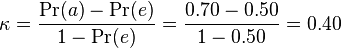
Note that there were 20 proposals that were granted by both reader A and reader B, and 15 proposals that were rejected by both readers. Thus, the observed proportionate agreement is Pr(a) = (20 + 15) / 50 = 0.70
To calculate Pr(e) (the probability of random agreement) we note that:
- Reader A said "Yes" to 25 applicants and "No" to 25 applicants. Thus reader A said "Yes" 50% of the time.
- Reader B said "Yes" to 30 applicants and "No" to 20 applicants. Thus reader B said "Yes" 60% of the time.
Therefore the probability that both of them would say "Yes" randomly is 0.50 · 0.60 = 0.30 and the probability that both of them would say "No" is 0.50 · 0.40 = 0.20. Thus the overall probability of random agreement is Pr(e) = 0.3 + 0.2 = 0.5.
So now applying our formula for Cohen's Kappa we get:
Same percentages but different numbers
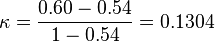
A case sometimes considered to be a problem with Cohen's Kappa occurs when comparing the Kappa calculated for two pairs of raters with the two raters in each pair having the same percentage agreement but one pair give a similar number of ratings while the other pair give a very different number of ratings.[8] For instance, in the following two cases there is equal agreement between A and B (60 out of 100 in both cases) so we would expect the relative values of Cohen's Kappa to reflect this. However, calculating Cohen's Kappa for each:
| B | |||
|---|---|---|---|
| Yes | No | ||
| A | Yes | 45 | 15 |
| No | 25 | 15 | |
| B | |||
|---|---|---|---|
| Yes | No | ||
| A | Yes | 25 | 35 |
| No | 5 | 35 | |
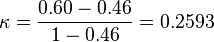
we find that it shows greater similarity between A and B in the second case, compared to the first. This is because while the percentage agreement is the same, the percentage agreement that would occur 'by chance' is significantly higher in the first case (0.54 compared to 0.46).
Significance and magnitude

Statistical significance makes no claim on how important is the magnitude in a given application or what is considered as high or low agreement.
Statistical significance for kappa is rarely reported, probably because even relatively low values of kappa can nonetheless be significantly different from zero but not of sufficient magnitude to satisfy investigators.[9]:66 Still, its standard error has been described[10] and is computed by various computer programs.[11]
If statistical significance is not a useful guide, what magnitude of kappa reflects adequate agreement? Guidelines would be helpful, but factors other than agreement can influence its magnitude, which makes interpretation of a given magnitude problematic. As Sim and Wright noted, two important factors are prevalence (are the codes equiprobable or do their probabilities vary) and bias (are the marginal probabilities for the two observers similar or different). Other things being equal, kappas are higher when codes are equiprobable. On the other hand Kappas are higher when codes are distributed asymmetrically by the two observers. In contrast to probability variations, the effect of bias is greater when Kappa is small than when it is large.[12]:261–262
Another factor is the number of codes. As number of codes increases, kappas become higher. Based on a simulation study, Bakeman and colleagues concluded that for fallible observers, values for kappa were lower when codes were fewer. And, in agreement with Sim & Wrights's statement concerning prevalence, kappas were higher when codes were roughly equiprobable. Thus Bakeman et al. concluded that "no one value of kappa can be regarded as universally acceptable."[13]:357 They also provide a computer program that lets users compute values for kappa specifying number of codes, their probability, and observer accuracy. For example, given equiprobable codes and observers who are 85% accurate, value of kappa are 0.49, 0.60, 0.66, and 0.69 when number of codes is 2, 3, 5, and 10, respectively.
Nonetheless, magnitude guidelines have appeared in the literature. Perhaps the first was Landis and Koch,[14] who characterized values < 0 as indicating no agreement and 0–0.20 as slight, 0.21–0.40 as fair, 0.41–0.60 as moderate, 0.61–0.80 as substantial, and 0.81–1 as almost perfect agreement. This set of guidelines is however by no means universally accepted; Landis and Koch supplied no evidence to support it, basing it instead on personal opinion. It has been noted that these guidelines may be more harmful than helpful.[15] Fleiss's[16]:218 equally arbitrary guidelines characterize kappas over 0.75 as excellent, 0.40 to 0.75 as fair to good, and below 0.40 as poor.
Weighted kappa
Weighted kappa lets you count disagreements differently[17] and is especially useful when codes are ordered.[9]:66 Three matrices are involved, the matrix of observed scores, the matrix of expected scores based on chance agreement, and the weight matrix. Weight matrix cells located on the diagonal (upper-left to bottom-right) represent agreement and thus contain zeros. Off-diagonal cells contain weights indicating the seriousness of that disagreement. Often, cells one off the diagonal are weighted 1, those two off 2, etc.
The equation for weighted κ is:
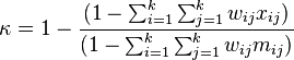
where k=number of codes and  ,
,  , and
, and  are elements in the weight, observed, and expected matrices, respectively. When diagonal cells contain weights of 0 and all off-diagonal cells weights of 1, this formula produces the same value of kappa as the calculation given above.
Kappa maximum
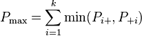
Kappa assumes its theoretical maximum value of 1 only when both observers distribute codes the same, that is, when corresponding row and column sums are identical. Anything less is less than perfect agreement. Still, the maximum value kappa could achieve given unequal distributions helps interpret the value of kappa actually obtained. The equation for κ maximum is:[18]
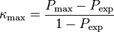
where 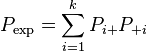 , as usual,
 ,
,
k = number of codes,  are the row probabilities, and
  are the column probabilities.
See also
References
- ↑ Carletta, Jean. (1996) Assessing agreement on classification tasks: The kappa statistic. Computational Linguistics, 22(2), pp. 249–254.
- ↑ Strijbos, J.; Martens, R.; Prins, F.; Jochems, W. (2006). "Content analysis: What are they talking about?". Computers & Education 46: 29–48. doi:10.1016/j.compedu.2005.04.002.
- ↑ Uebersax, JS. (1987). "Diversity of decision-making models and the measurement of interrater agreement" (PDF). Psychological Bulletin 101: 140–146. doi:10.1037/0033-2909.101.1.140.
- ↑ Galton, F. (1892). Finger Prints Macmillan, London.
- ↑ Smeeton, N.C. (1985). "Early History of the Kappa Statistic". Biometrics 41: 795.
- ↑ Cohen, Jacob (1960). "A coefficient of agreement for nominal scales". Educational and Psychological Measurement 20 (1): 37–46. doi:10.1177/001316446002000104
- ↑ Powers, David M. W. (2012). "The Problem with Kappa" (PDF). Conference of the European Chapter of the Association for Computational Linguistics (EACL2012) Joint ROBUS-UNSUP Workshop.
- ↑ Kilem Gwet (May 2002). "Inter-Rater Reliability: Dependency on Trait Prevalence and Marginal Homogeneity" (PDF). Statistical Methods for Inter-Rater Reliability Assessment 2: 1–10.
- ↑ 9.0 9.1 Bakeman, R.; Gottman, J.M. (1997). Observing interaction: An introduction to sequential analysis (2nd ed.). Cambridge, UK: Cambridge University Press. ISBN 0-521-27593-8.
- ↑ Fleiss, J.L.; Cohen, J.; Everitt, B.S. (1969). "Large sample standard errors of kappa and weighted kappa". Psychological Bulletin 72: 323–327. doi:10.1037/h0028106.
- ↑ Robinson, B.F; Bakeman, R. (1998). "ComKappa: A Windows 95 program for calculating kappa and related statistics". Behavior Research Methods, Instruments, and Computers 30: 731–732. doi:10.3758/BF03209495.
- ↑ Sim, J; Wright, C. C (2005). "The Kappa Statistic in Reliability Studies: Use, Interpretation, and Sample Size Requirements". Physical Therapy 85: 257–268. PMID 15733050.
- ↑ Bakeman, R.; Quera, V.; McArthur, D.; Robinson, B. F. (1997). "Detecting sequential patterns and determining their reliability with fallible observers". Psychological Methods 2: 357–370. doi:10.1037/1082-989X.2.4.357.
- ↑ Landis, J.R.; Koch, G.G. (1977). "The measurement of observer agreement for categorical data". Biometrics 33 (1): 159–174. doi:10.2307/2529310. JSTOR 2529310. PMID 843571.
- ↑ Gwet, K. (2010). "Handbook of Inter-Rater Reliability (Second Edition)" ISBN 978-0-9708062-2-2
- ↑ Fleiss, J.L. (1981). Statistical methods for rates and proportions (2nd ed.). New York: John Wiley. ISBN 0-471-26370-2.
- ↑ Cohen, J. (1968). "Weighed kappa: Nominal scale agreement with provision for scaled disagreement or partial credit". Psychological Bulletin 70 (4): 213–220. doi:10.1037/h0026256. PMID 19673146.
- ↑ Umesh, U. N.; Peterson, R.A., & Sauber. M. H. (1989). "Interjudge agreement and the maximum value of kappa.". Educational and Psychological Measurement 49: 835–850. doi:10.1177/001316448904900407.
Further reading
- Banerjee, M.; Capozzoli, Michelle; McSweeney, Laura; Sinha, Debajyoti (1999). "Beyond Kappa: A Review of Interrater Agreement Measures". The Canadian Journal of Statistics / La Revue Canadienne de Statistique 27 (1): 3–23. JSTOR 3315487.
- Brennan, R. L.; Prediger, D. J. (1981). "Coefficient λ: Some Uses, Misuses, and Alternatives". Educational and Psychological Measurement 41: 687–699. doi:10.1177/001316448104100307.
- Cohen, Jacob (1960). "A coefficient of agreement for nominal scales". Educational and Psychological Measurement 20 (1): 37–46. doi:10.1177/001316446002000104.
- Cohen, J. (1968). "Weighted kappa: Nominal scale agreement with provision for scaled disagreement or partial credit". Psychological Bulletin 70 (4): 213–220. doi:10.1037/h0026256. PMID 19673146.
- Fleiss, J.L. (1971). "Measuring nominal scale agreement among many raters". Psychological Bulletin 76 (5): 378–382. doi:10.1037/h0031619.
- Fleiss, J. L. (1981) Statistical methods for rates and proportions. 2nd ed. (New York: John Wiley) pp. 38–46
- Fleiss, J.L.; Cohen, J. (1973). "The equivalence of weighted kappa and the intraclass correlation coefficient as measures of reliability". Educational and Psychological Measurement 33: 613–619. doi:10.1177/001316447303300309.
- Gwet, Kilem L. (2014) Handbook of Inter-Rater Reliability, Fourth Edition, (Gaithersburg : Advanced Analytics, LLC) ISBN 978-0970806284
- Gwet, K. (2008). "Computing inter-rater reliability and its variance in the presence of high agreement" (PDF). British Journal of Mathematical and Statistical Psychology 61 (Pt 1): 29–48. doi:10.1348/000711006X126600. PMID 18482474.
- Gwet, K. (2008). "Variance Estimation of Nominal-Scale Inter-Rater Reliability with Random Selection of Raters" (PDF). Psychometrika 73 (3): 407–430. doi:10.1007/s11336-007-9054-8.
- Gwet, K. (2008). "Intrarater Reliability." Wiley Encyclopedia of Clinical Trials, Copyright 2008 John Wiley & Sons, Inc.
- Scott, W. (1955). "Reliability of content analysis: The case of nominal scale coding". Public Opinion Quarterly 17: 321–325.
- Sim, J.; Wright, C. C. (2005). "The Kappa Statistic in Reliability Studies: Use, Interpretation, and Sample Size Requirements". Physical Therapy 85 (3): 257–268. PMID 15733050.
External links
- The Problem with Kappa
- Kappa, its meaning, problems, and several alternatives
- Kappa Statistics: Pros and Cons
- Windows program for kappa, weighted kappa, and kappa maximum
- Java and PHP implementation of weighted Kappa
Online calculators
- Cohen's Kappa for Maps
- Online (Multirater) Kappa Calculator
- Online Kappa Calculator (multiple raters and variables)
- Vassar College's Kappa Calculator
- NIWA's Cohen's Kappa Calculator
| ||||||||||||||||||||||||||||||||||||||||||||||||||||||||||||||||||||||||||||||||||||||||||||||||||||||||||||||||||||||||||||||||||||||||||||||||||||||||||||||||||||||||||||||||||||||||||||||||||||||||||||||||||||||