Coefficient of determination


In statistics, the coefficient of determination, denoted R2 or r2 and pronounced R squared, is a number that indicates how well data fit a statistical model – sometimes simply a line or curve. It is a statistic used in the context of statistical models whose main purpose is either the prediction of future outcomes or the testing of hypotheses, on the basis of other related information. It provides a measure of how well observed outcomes are replicated by the model, as the proportion of total variation of outcomes explained by the model (pp. 187, 287).[1][2][3]
There are several definitions of R2 that are only sometimes equivalent. One class of such cases includes that of simple linear regression where r2 is used instead of R2. In this case, if an intercept is included, then r2 is simply the square of the sample correlation coefficient (i.e., r) between the outcomes and their predicted values. If additional explanators are included, R2 is the square of the coefficient of multiple correlation. In both such cases, the coefficient of determination ranges from 0 to 1.
Important cases where the computational definition of R2 can yield negative values, depending on the definition used, arise where the predictions that are being compared to the corresponding outcomes have not been derived from a model-fitting procedure using those data, and where linear regression is conducted without including an intercept. Additionally, negative values of R2 may occur when fitting non-linear functions to data.[4] In cases where negative values arise, the mean of the data provides a better fit to the outcomes than do the fitted function values, according to this particular criterion.[5]
Definitions

The better the linear regression (on the right) fits the data in comparison to the simple average (on the left graph), the closer the value of
 is to 1. The areas of the blue squares represent the squared residuals with respect to the linear regression. The areas of the red squares represent the squared residuals with respect to the average value.
A data set has n values marked y1...yn (collectively known as yi), each associated with a predicted (or modeled) value f1...fn (known as fi, or sometimes ŷi).
If  is the mean of the observed data:

then the variability of the data set can be measured using three sums of squares formulas:
- The total sum of squares (proportional to the variance of the data):
- The regression sum of squares, also called the explained sum of squares:
- The sum of squares of residuals, also called the residual sum of squares:
The notations  and
and  should be avoided, since in some texts their meaning is reversed to Residual sum of squares and Explained sum of squares, respectively.
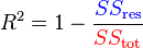
The most general definition of the coefficient of determination is
Relation to unexplained variance
In a general form, R2 can be seen to be related to the unexplained variance, since the second term compares the unexplained variance (variance of the model's errors) with the total variance (of the data). See fraction of variance unexplained.
As explained variance
In some cases the total sum of squares equals the sum of the two other sums of squares defined above,

See partitioning in the general OLS model for a derivation of this result for one case where the relation holds. When this relation does hold, the above definition of R2 is equivalent to
In this form R2 is expressed as the ratio of the explained variance (variance of the model's predictions, which is SSreg / n) to the total variance (sample variance of the dependent variable, which is SStot / n).
This partition of the sum of squares holds for instance when the model values ƒi have been obtained by linear regression. A milder sufficient condition reads as follows: The model has the form

where the qi are arbitrary values that may or may not depend on i or on other free parameters (the common choice qi = xi is just one special case), and the coefficients α and β are obtained by minimizing the residual sum of squares.
This set of conditions is an important one and it has a number of implications for the properties of the fitted residuals and the modelled values. In particular, under these conditions:

As squared correlation coefficient
Similarly, in linear least squares regression with an estimated intercept term, R2 equals the square of the Pearson correlation coefficient between the observed and modeled (predicted) data values of the dependent variable.
Under more general modeling conditions, where the predicted values might be generated from a model different from linear least squares regression, an R2 value can be calculated as the square of the correlation coefficient between the original and modeled data values. In this case, the value is not directly a measure of how good the modeled values are, but rather a measure of how good a predictor might be constructed from the modeled values (by creating a revised predictor of the form α + βƒi). According to Everitt (p. 78),[6] this usage is specifically the definition of the term "coefficient of determination": the square of the correlation between two (general) variables.
Interpretation
R2 is a statistic that will give some information about the goodness of fit of a model. In regression, the R2 coefficient of determination is a statistical measure of how well the regression line approximates the real data points. An R2 of 1 indicates that the regression line perfectly fits the data.
Values of R2 outside the range 0 to 1 can occur where it is used to measure the agreement between observed and modeled values and where the "modeled" values are not obtained by linear regression and depending on which formulation of R2 is used. If the first formula above is used, values can be less than zero. If the second expression is used, values can be greater than one. Neither formula is defined for the case where  .
.
In many (but not all) instances where R2 is used, the predictors are calculated by ordinary least-squares regression: that is, by minimizing SSres. In this case R2 increases as we increase the number of variables in the model (R2 is monotone increasing with the number of variables included—i.e., it will never decrease). This illustrates a drawback to one possible use of R2, where one might keep adding variables (Kitchen sink regression) to increase the R2 value. For example, if one is trying to predict the sales of a model of car from the car's gas mileage, price, and engine power, one can include such irrelevant factors as the first letter of the model's name or the height of the lead engineer designing the car because the R2 will never decrease as variables are added and will probably experience an increase due to chance alone.
This leads to the alternative approach of looking at the adjusted R2. The explanation of this statistic is almost the same as R2 but it penalizes the statistic as extra variables are included in the model. For cases other than fitting by ordinary least squares, the R2 statistic can be calculated as above and may still be a useful measure. If fitting is by weighted least squares or generalized least squares, alternative versions of R2 can be calculated appropriate to those statistical frameworks, while the "raw" R2 may still be useful if it is more easily interpreted. Values for R2 can be calculated for any type of predictive model, which need not have a statistical basis.
In a non-simple linear model
Consider a linear model with more than a single explanatory variable, of the form
where, for the ith case,  is the response variable,
  are p regressors, and
  is a mean zero error term. The quantities
  are unknown coefficients, whose values are estimated by least squares. The coefficient of determination R2 is a measure of the global fit of the model. Specifically, R2 is an element of [0, 1] and represents the proportion of variability in Yi that may be attributed to some linear combination of the regressors (explanatory variables) in X.
R2 is often interpreted as the proportion of response variation "explained" by the regressors in the model. Thus, R2 = 1 indicates that the fitted model explains all variability in  , while R2 = 0 indicates no 'linear' relationship (for straight line regression, this means that the straight line model is a constant line (slope = 0, intercept = ) between the response variable and regressors). An interior value such as R2 = 0.7 may be interpreted as follows: "Seventy percent of the variance in the response variable can be explained by the explanatory variables. The remaining thirty percent can be attributed to unknown, lurking variables or inherent variability."
A caution that applies to R2, as to other statistical descriptions of correlation and association is that "correlation does not imply causation." In other words, while correlations may provide valuable clues regarding causal relationships among variables, a high correlation between two variables does not represent adequate evidence that changing one variable has resulted, or may result, from changes of other variables.
In case of a single regressor, fitted by least squares, R2 is the square of the Pearson product-moment correlation coefficient relating the regressor and the response variable. More generally, R2 is the square of the correlation between the constructed predictor and the response variable. With more than one regressor, the R2 can be referred to as the coefficient of multiple determination.
Inflation of R2
In least squares regression, R2 is weakly increasing with increases in the number of regressors in the model. Because increases in the number of regressors increase the value of R2, R2 alone cannot be used as a meaningful comparison of models with very different numbers of independent variables. For a meaningful comparison between two models, an F-test can be performed on the residual sum of squares, similar to the F-tests in Granger causality, though this is not always appropriate. As a reminder of this, some authors denote R2 by Rp2, where p is the number of columns in X (the number of explanators including the constant).
To demonstrate this property, first recall that the objective of least squares linear regression is:
The optimal value of the objective is weakly smaller as additional columns of  are added, by the fact that less constrained minimization leads to an optimal cost which is weakly smaller than more constrained minimization does. Given the previous conclusion and noting that
  depends only on y, the non-decreasing property of R2 follows directly from the definition above.
The intuitive reason that using an additional explanatory variable cannot lower the R2 is this: Minimizing  is equivalent to maximizing R2. When the extra variable is included, the data always have the option of giving it an estimated coefficient of zero, leaving the predicted values and the R2 unchanged. The only way that the optimization problem will give a non-zero coefficient is if doing so improves the R2.
Notes on interpreting R2
R2 does not indicate whether:
- the independent variables are a cause of the changes in the dependent variable;
- omitted-variable bias exists;
- the correct regression was used;
- the most appropriate set of independent variables has been chosen;
- there is collinearity present in the data on the explanatory variables;
- the model might be improved by using transformed versions of the existing set of independent variables;
- there are enough data points to make a solid conclusion.
Adjusted R2
The use of an adjusted R2 (often written as  and pronounced "R bar squared") is an attempt to take account of the phenomenon of the R2 automatically and spuriously increasing when extra explanatory variables are added to the model. It is a modification due to Theil[7] of R2 that adjusts for the number of explanatory terms in a model relative to the number of data points. The adjusted R2 can be negative, and its value will always be less than or equal to that of R2. Unlike R2, the adjusted R2 increases when a new explanator is included only if the new explanator improves the R2 more than would be expected by chance. If a set of explanatory variables with a predetermined hierarchy of importance are introduced into a regression one at a time, with the adjusted R2 computed each time, the level at which adjusted R2 reaches a maximum, and decreases afterward, would be the regression with the ideal combination of having the best fit without excess/unnecessary terms. The adjusted R2 is defined as

where p is the total number of regressors in the model (not counting the constant term), and n is the sample size.
Adjusted R2 can also be written as
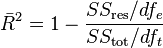
where dft is the degrees of freedom n– 1 of the estimate of the population variance of the dependent variable, and dfe is the degrees of freedom n – p – 1 of the estimate of the underlying population error variance.
The principle behind the adjusted R2 statistic can be seen by rewriting the ordinary R2 as
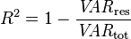
where  and
and  are the sample variances of the estimated residuals and the dependent variable respectively, which can be seen as biased estimates of the population variances of the errors and of the dependent variable. These estimates are replaced by statistically unbiased versions:
  and
and  .
.
Adjusted R2 does not have the same interpretation as R2—while R2 is a measure of fit, adjusted R2 is instead a comparative measure of suitability of alternative nested sets of explanators. As such, care must be taken in interpreting and reporting this statistic. Adjusted R2 is particularly useful in the feature selection stage of model building.
Generalized R2
The generalized R² was originally proposed by Cox & Snell,[8] and independently by Magee:[9]
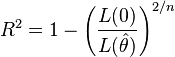
where L(0) is the likelihood of the model with only the intercept,  is the likelihood of the estimated model (i.e., the model with a given set of parameter estimates) and n is the sample size.
Nagelkerke[10] noted that it had the following properties:
- It's consistent with the classical coefficient of determination when both can be computed;
- Its value is maximised by the maximum likelihood estimation of a model;
- It is asymptotically independent of the sample size;
- The interpretation is the proportion of the variation explained by the model;
- The values are between 0 and 1, with 0 denoting that model does not explain any variation and 1 denoting that it perfectly explains the observed variation;
- It does not have any unit.
However, in the case of a logistic model, where  cannot be greater than 1, R² is between 0 and
 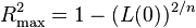 : thus, Nagelkerke suggests the possibility to define a scaled R² as R²/R²max.[11]
Comparison with norm of residuals
Occasionally the norm of residuals is used for indicating goodness of fit. This term is encountered in MATLAB and is calculated by

Both R2 and the norm of residuals have their relative merits. For least squares analysis R2 varies between 0 and 1, with larger numbers indicating better fits and 1 represents a perfect fit. Norm of residuals varies from 0 to infinity with smaller numbers indicating better fits and zero indicating a perfect fit. One advantage and disadvantage of R2 is the  term acts to normalize the value. If the yi values are all multiplied by a constant, the norm of residuals will also change by that constant but R2 will stay the same. As a basic example, for the linear least squares fit to the set of data:


R2 = 0.998, and norm of residuals = 0.302. If all values of y are multiplied by 1000 (for example, in an SI prefix change), then R2 remains the same, but norm of residuals = 302.
See also
- Fraction of variance unexplained
- Goodness of fit
- Nash–Sutcliffe model efficiency coefficient (hydrological applications)
- Pearson product-moment correlation coefficient
- Proportional reduction in loss
- Regression model validation
- Root mean square deviation
- t-test of

Notes
- ↑ Steel, R. G. D.; Torrie, J. H. (1960). Principles and Procedures of Statistics with Special Reference to the Biological Sciences. McGraw Hill.
- ↑ Glantz, Stanton A.; Slinker, B. K. (1990). Primer of Applied Regression and Analysis of Variance. McGraw-Hill. ISBN 0-07-023407-8.
- ↑ Draper, N. R.; Smith, H. (1998). Applied Regression Analysis. Wiley-Interscience. ISBN 0-471-17082-8.
- ↑ Colin Cameron, A.; Windmeijer, Frank A.G.; Gramajo, H; Cane, DE; Khosla, C (1997). "An R-squared measure of goodness of fit for some common nonlinear regression models". Journal of Econometrics 77 (2): 1790–2. doi:10.1016/S0304-4076(96)01818-0. PMID 11230695.
- ↑ Imdadullah, Muhammad. "Coefficient of Determination". itfeature.com.
- ↑ Everitt, B. S. (2002). Cambridge Dictionary of Statistics (2nd ed.). CUP. ISBN 0-521-81099-X.
- ↑ Theil, Henri (1961). Economic Forecasts and Policy. Holland, Amsterdam: North.
- ↑ Cox, D. D.; Snell, E. J. (1989). The Analysis of Binary Data (2nd ed.). Chapman and Hall.
- ↑ Magee, L. (1990). "R2 measures based on Wald and likelihood ratio joint significance tests". The American Statistician 44. pp. 250–3. doi:10.1080/00031305.1990.10475731.
- ↑ Nagelkerke, Nico J. D. (1992). Maximum Likelihood Estimation of Functional Relationships, Pays-Bas. Lecture Notes in Statistics 69. ISBN 0-387-97721-X.
- ↑ Nagelkerke, N. J. D. (1991). "A Note on a General Definition of the Coefficient of Determination". Biometrika 78 (3): 691–2. doi:10.1093/biomet/78.3.691. JSTOR 2337038.
References
- Gujarati, Damodar N.; Porter, Dawn C. (2009). Basic Econometrics (Fifth ed.). New York: McGraw-Hill/Irwin. pp. 73–78. ISBN 978-0-07-337577-9.
- Kmenta, Jan (1986). Elements of Econometrics (Second ed.). New York: Macmillan. pp. 240–243. ISBN 0-02-365070-2.