Cochran's theorem

In statistics, Cochran's theorem, devised by William G. Cochran,^[1] is a theorem used to justify results relating to the probability distributions of statistics that are used in the analysis of variance.^[2]

Statement

Suppose U₁, ..., U_n are independent standard normally distributed random variables, and an identity of the form

\sum_{i=1}^n U_i^2=Q_1+\cdots + Q_k

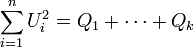
can be written, where each Q_i is a sum of squares of linear combinations of the Us. Further suppose that

r_1+\cdots +r_k=n

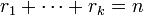
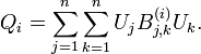
where r_i is the rank of Q_i. Cochran's theorem states that the Q_i are independent, and each Q_i has a chi-squared distribution with r_i degrees of freedom.^[1] Here the rank of Q_i should be interpreted as meaning the rank of the matrix B⁽ⁱ⁾, with elements B_j,k⁽ⁱ⁾, in the representation of Q_i as a quadratic form:

Q_i=\sum_{j=1}^n\sum_{k=1}^n U_j B_{j,k}^{(i)} U_k .

Less formally, it is the number of linear combinations included in the sum of squares defining Q_i, provided that these linear combinations are linearly independent.

Proof

We first show that the matrices B⁽ⁱ⁾ can be simultaneously diagonalized and that their non-zero eigenvalues are all equal to +1. We then use the vector basis that diagonalize them to simplify their characteristic function and show their independence and distribution.^[3]

Each of the matrices B⁽ⁱ⁾ has rank r_i and so has exactly r_i non-zero eigenvalues. For each i, the sum 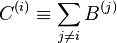$C^{(i)} \equiv \sum_{j\ne i}B^{(j)}$ has at most rank 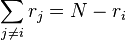$\sum_{j\ne i}r_j = N-r_i$ . Since 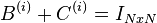$B^{(i)}+C^{(i)} = I_{NxN}$ , it follows that C⁽ⁱ⁾ has exactly rank N-r_i.

Therefore B⁽ⁱ⁾ and C⁽ⁱ⁾ can be simultaneously diagonalized. This can be shown by first diagonalizing B⁽ⁱ⁾. In this basis, it is of the form:

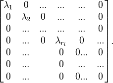
\begin{bmatrix} \lambda_1 & 0 & ... & ... & ... &0 \\ 0 & \lambda_2 & 0 & ... & ... & 0 \\ 0 & ... & ... & ... & ... & 0\\ 0 & ... &0 & \lambda_{r_i} & 0 &... \\ 0 & ... & & 0 & 0...&0\\ 0 & ... & & 0 & ...&...\\ 0 & ... & & 0 & 0...&0 \end{bmatrix}.

Thus the lower $(N-r_i)$ rows are zero. Since 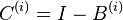$C^{(i)} = I - B^{(i)}$ , it follows these rows in C⁽ⁱ⁾ in this basis contain a right block which is a 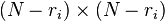$(N-r_i)\times(N-r_i)$ unit matrix, with zeros in the rest of these rows. But since C⁽ⁱ⁾ has rank N-r_i, it must be zero elsewhere. Thus it is diagonal in this basis as well. Moreover, it follows that all the non-zero eigenvalues of both B⁽ⁱ⁾ and C⁽ⁱ⁾ are +1.

It follows that the non-zero eigenvalues of all the B-s are equal to +1. Moreover, the above analysis can be repeated in the diagonal basis for 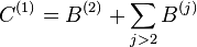$C^{(1)} = B^{(2)} + \sum_{j>2}B^{(j)}$ . In this basis $C^{(1)}$ is the identity of an $(N-r_i)\times(N-r_i)$ vector space, so it follows that both B⁽²⁾ and $\sum_{j>2}B^{(j)}$ are simultaneously diagonalizable in this vector space (and hence also together B⁽¹⁾). By repeating this over and over it follows that all the B-s are simultaneously diagonalizable.

Thus there exists an orthogonal matrix S such that for all i between 1 and k: $S^\mathrm{T}Q_i S$ is diagonal with the diagonal having 1-s at the places between $r_1 + ... r_{i-1} +1$ and $r_1 + ... r_i$ .

Let $U_i^\prime$ be the independent variables $U_i$ after transformation by S.

The characteristic function of Q_i is:

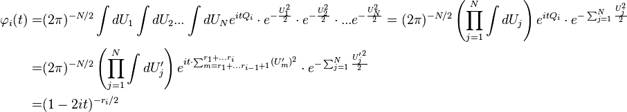
\begin{align} \varphi_i(t) =& (2\pi)^{-N/2} \int dU_1 \int dU_2 ... \int dU_N e^{i t Q_i} \cdot e^{-\frac{U_1^2}{2}}\cdot e^{-\frac{U_2^2}{2}}\cdot ...e^{-\frac{U_N^2}{2}} = (2\pi)^{-N/2} \left(\prod_{j=1}^N \int dU_j\right) e^{i t Q_i} \cdot e^{-\sum_{j=1}^N \frac{U_j^2}{2}} \\ =& (2\pi)^{-N/2} \left(\prod_{j=1}^N \int dU_j^\prime\right) e^{i t\cdot \sum_{m = r_1+...r_{i-1}+1}^{r_1+...r_i} (U_m^\prime)^2} \cdot e^{-\sum_{j=1}^N \frac{{U_j^\prime}^2}{2}} \\ =& (1 - 2 i t)^{-r_i/2} \end{align}

This is the Fourier transform of the chi-squared distribution with r_i degrees of freedom. Therefore this is the distribution of Q_i.

Moreover, the characteristic function of the joint distribution of all the Q_i-s is:

\begin{align} \varphi(t_1, t_2... t_k) =& (2\pi)^{-N/2} \left(\prod_{j=1}^N \int dU_j\right) e^{i \sum_{i=1}^k t_i \cdot Q_i} \cdot e^{-\sum_{j=1}^N \frac{U_j^2}{2}} \\ =& (2\pi)^{-N/2} \left(\prod_{j=1}^N \int dU_j^\prime\right) e^{i \cdot \sum_{i=1}^k t_i \sum_{k = r_1+...r_{i-1}+1}^{r_1+...r_i} (U_k^\prime)^2} \cdot e^{-\sum_{j=1}^N \frac{{U_j^\prime}^2}{2}} \\ =& \prod_{i=1}^k (1 - 2 i t_i)^{-r_i/2} = \prod_{i=1}^k \varphi_i(t_i) \end{align}

From which it follows that all the Q_i-s are statistically independent.

Examples

Sample mean and sample variance

If X₁, ..., X_n are independent normally distributed random variables with mean μ and standard deviation σ then

U_i = \frac{X_i-\mu}{\sigma}

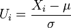
is standard normal for each i. It is possible to write

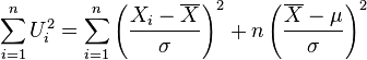
\sum_{i=1}^n U_i^2=\sum_{i=1}^n\left(\frac{X_i-\overline{X}}{\sigma}\right)^2 + n\left(\frac{\overline{X}-\mu}{\sigma}\right)^2

(here $\overline{X}$ is the sample mean). To see this identity, multiply throughout by $\sigma^2$ and note that

\sum(X_i-\mu)^2= \sum(X_i-\overline{X}+\overline{X}-\mu)^2

and expand to give

\sum(X_i-\mu)^2= \sum(X_i-\overline{X})^2+\sum(\overline{X}-\mu)^2+ 2\sum(X_i-\overline{X})(\overline{X}-\mu).

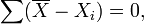
The third term is zero because it is equal to a constant times

\sum(\overline{X}-X_i)=0,

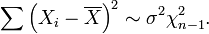
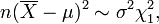
and the second term has just n identical terms added together. Thus

\sum(X_i-\mu)^2= \sum(X_i-\overline{X})^2+n(\overline{X}-\mu)^2 ,

and hence

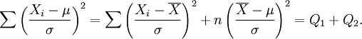
\sum\left(\frac{X_i-\mu}{\sigma}\right)^2= \sum\left(\frac{X_i-\overline{X}}{\sigma}\right)^2 +n\left(\frac{\overline{X}-\mu}{\sigma}\right)^2 =Q_1+Q_2.

Now the rank of Q₂ is just 1 (it is the square of just one linear combination of the standard normal variables). The rank of Q₁ can be shown to be n − 1, and thus the conditions for Cochran's theorem are met.

Cochran's theorem then states that Q₁ and Q₂ are independent, with chi-squared distributions with n − 1 and 1 degree of freedom respectively. This shows that the sample mean and sample variance are independent. This can also be shown by Basu's theorem, and in fact this property characterizes the normal distribution – for no other distribution are the sample mean and sample variance independent.^[4]

Distributions

The result for the distributions is written symbolically as

\sum\left(X_i-\overline{X}\right)^2 \sim \sigma^2 \chi^2_{n-1}.

n(\overline{X}-\mu)^2\sim \sigma^2 \chi^2_1,

Both these random variables are proportional to the true but unknown variance σ². Thus their ratio does not depend on σ² and, because they are statistically independent. The distribution of their ratio is given by

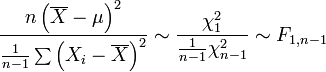
\frac{n\left(\overline{X}-\mu\right)^2} {\frac{1}{n-1}\sum\left(X_i-\overline{X}\right)^2}\sim \frac{\chi^2_1}{\frac{1}{n-1}\chi^2_{n-1}} \sim F_{1,n-1}

where F_1,n − 1 is the F-distribution with 1 and n − 1 degrees of freedom (see also Student's t-distribution). The final step here is effectively the definition of a random variable having the F-distribution.

Estimation of variance

To estimate the variance σ², one estimator that is sometimes used is the maximum likelihood estimator of the variance of a normal distribution

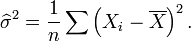
\widehat{\sigma}^2= \frac{1}{n}\sum\left( X_i-\overline{X}\right)^2.

Cochran's theorem shows that

\frac{n\widehat{\sigma}^2}{\sigma^2}\sim\chi^2_{n-1}

and the properties of the chi-squared distribution show that the expected value of $\widehat{\sigma}^2$ is σ²(n − 1)/n.

Alternative formulation

The following version is often seen when considering linear regression. Suppose that $Y\sim N_n(0,\sigma^2I_n)$ is a standard multivariate normal random vector (here $I_n$ denotes the n-by-n identity matrix), and if $A_1,\ldots,A_k$ are all n-by-n symmetric matrices with $\sum_{i=1}^kA_i=I_n$ . Then, on defining $r_i=Rank(A_i)$ , any one of the following conditions implies the other two:

$\sum_{i=1}^kr_i=n ,$
$Y^TA_iY\sim\sigma^2\chi^2_{r_i}$ (thus the $A_i$ are positive semidefinite)
$Y^TA_iY$ is independent of $Y^TA_jY$ for $i\neq j .$

References

↑ 1.0 1.1 Cochran, W. G. (April 1934). "The distribution of quadratic forms in a normal system, with applications to the analysis of covariance". Mathematical Proceedings of the Cambridge Philosophical Society 30 (2): 178–191. doi:10.1017/S0305004100016595.
↑ Bapat, R. B. (2000). Linear Algebra and Linear Models (Second ed.). Springer. ISBN 978-0-387-98871-9.
↑ Craig A.T. (1938) On The Independence of Certain Estimates of Variances. Ann. Math. Statist. 9, pp. 48-55
↑ Geary, R.C. (1936). "The Distribution of the "Student's" Ratio for the Non-Normal Samples". Supplement to the Journal of the Royal Statistical Society 3 (2): 178–184. doi:10.2307/2983669. JFM 63.1090.03. JSTOR 2983669.

Design of experiments

Scientific method	Scientific experiment Statistical design Control Internal and external validity Experimental unit Blinding Optimal design: Bayesian Random assignment Randomization Restricted randomization Replication versus subsampling Sample size

Treatment and blocking	Treatment Effect size Contrast Interaction Confounding Orthogonality Blocking Covariate Nuisance variable

Models and inference	Linear regression Ordinary least squares Bayesian Random effect Mixed model Hierarchical model: Bayesian Analysis of variance (Anova) Cochran's theorem Manova (multivariate) Ancova (covariance) Compare means Multiple comparison

Designs Completely randomized	Factorial Fractional factorial Plackett-Burman Taguchi Response surface methodology Polynomial and rational modeling Box-Behnken Central composite Block Generalized randomized block design (GRBD) Latin square Graeco-Latin square Orthogonal array Latin hypercube Repeated measures design Crossover study Randomized controlled trial Sequential analysis Sequential probability ratio test

Glossary Category Statistics portal Statistical outline Statistical topics