Chi-squared test
A chi-squared test, also referred to as  test (or chi-square test), is any statistical hypothesis test in which the sampling distribution of the test statistic is a chi-squared distribution when the null hypothesis is true. Also considered a chi-squared test is a test in which this is asymptotically true, meaning that the sampling distribution (if the null hypothesis is true) can be made to approximate a chi-squared distribution as closely as desired by making the sample size large enough.
The chi-squared (I) test is used to determine whether there is a significant difference between the expected
frequencies and the observed frequencies in one or more categories. Does the number of individuals or objects that
fall in each category differ significantly from the number you would expect? Is this difference between the
expected and observed due to sampling variation, or is it a real difference?
test (or chi-square test), is any statistical hypothesis test in which the sampling distribution of the test statistic is a chi-squared distribution when the null hypothesis is true. Also considered a chi-squared test is a test in which this is asymptotically true, meaning that the sampling distribution (if the null hypothesis is true) can be made to approximate a chi-squared distribution as closely as desired by making the sample size large enough.
The chi-squared (I) test is used to determine whether there is a significant difference between the expected
frequencies and the observed frequencies in one or more categories. Does the number of individuals or objects that
fall in each category differ significantly from the number you would expect? Is this difference between the
expected and observed due to sampling variation, or is it a real difference?
Examples of chi-squared tests with samples
The following are examples of chi-squared tests where the chi-squared distribution is approximately valid:
Pearson's chi-squared test
Pearson's chi-squared test, also known as the chi-squared goodness-of-fit test or chi-squared test for independence. When the chi-squared test is mentioned without any modifiers or without other precluding context, this test is often meant (for an exact test used in place of , see Fisher's exact test).
Yates's correction for continuity
Using the chi-squared distribution to interpret Pearson's chi-squared statistic requires one to assume that the discrete probability of observed binomial frequencies in the table can be approximated by the continuous chi-squared distribution. This assumption is not quite correct, and introduces some error.
To reduce the error in approximation, Frank Yates suggested a correction for continuity that adjusts the formula for Pearson's chi-squared test by subtracting 0.5 from the difference between each observed value and its expected value in a 2 × 2 contingency table.[1] This reduces the chi-squared value obtained and thus increases its p-value.
Other chi-squared tests
- Cochran–Mantel–Haenszel chi-squared test.
- McNemar's test, used in certain 2 × 2 tables with pairing
- Tukey's test of additivity
- The portmanteau test in time-series analysis, testing for the presence of autocorrelation
- Likelihood-ratio tests in general statistical modelling, for testing whether there is evidence of the need to move from a simple model to a more complicated one (where the simple model is nested within the complicated one).
Exact chi-squared distribution
One case where the distribution of the test statistic is an exact chi-squared distribution is the test that the variance of a normally distributed population has a given value based on a sample variance. Such a test is uncommon in practice because values of variances to test against are seldom known exactly.
Chi-squared test for variance in a normal population
If a sample of size n is taken from a population having a normal distribution, then there is a result (see distribution of the sample variance) which allows a test to be made of whether the variance of the population has a pre-determined value. For example, a manufacturing process might have been in stable condition for a long period, allowing a value for the variance to be determined essentially without error. Suppose that a variant of the process is being tested, giving rise to a small sample of n product items whose variation is to be tested. The test statistic T in this instance could be set to be the sum of squares about the sample mean, divided by the nominal value for the variance (i.e. the value to be tested as holding). Then T has a chi-squared distribution with n − 1 degrees of freedom. For example if the sample size is 21, the acceptance region for T for a significance level of 5% is the interval 9.59 to 34.17.
Chi-squared test for independence and homogeneity in tables
Suppose a random sample of 650 of the 1 million residents of a city is taken, in which every resident of each of four neighborhoods, A, B, C, and D, is equally likely to be chosen. A null hypothesis says the randomly chosen person's neighborhood of residence is independent of the person's occupational classification, which is either "blue collar", "white collar", or "service". The data are tabulated:
![\begin{array}{l|c|c|c|c|c|c}
& \text{A} & \text{B} & \text{C} & \text{D} & & \text{total} \\[6pt]
\hline
\text{Blue collar} & 90 & 60 & 104 & 95 & & 349 \\[6pt]
\hline
\text{White collar} & 30 & 50 & 51 & 20 & & 151 \\[6pt]
\hline
\text{Service} & 30 & 40 & 45 & 35 & & 150 \\[12pt]
\hline
\text{total} & 150 & 150 & 200 & 150 & & 650
\end{array}](../I/m/926a90f40981f23b62585c32dd259b98.png)
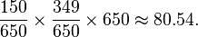
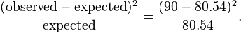
Let us take the sample proportion living in neighborhood A, 150/650, to estimate what proportion of the whole 1 million people live in neighborhood A. Similarly we take 349/650 to estimate what proportion of the 1 million people are blue-collar workers. Then the null hypothesis independence tells us that we should "expect" the number of blue-collar workers in neighborhood A to be
Then in that "cell" of the table, we have
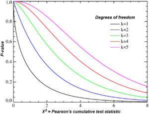
The sum of these quantities over all of the cells is the test statistic. Under the null hypothesis, it has approximately a chi-squared distribution whose number of degrees of freedom is

If the test statistic is improbably large according to that chi-squared distribution, then one rejects the null hypothesis of independence.
A related issue is a test of homogeneity. Suppose that instead of giving every resident of each of the four neighborhoods an equal chance of inclusion in the sample, we decide in advance how many residents of each neighborhood to include. Then each resident has the same chance of being chosen as do all residents of the same neighborhood, but residents of different neighborhoods would have different probabilities of being chosen if the four sample sizes are not proportional to the populations of the four neighborhoods. In such a case, we would be testing "homogeneity" rather than "independence". The question is whether the proportions of blue-collar, white-collar, and service workers in the four neighborhoods are the same. However, the test is done in the same way.
Applications
In cryptanalysis, chi-squared test is used to compare the distribution of plaintext and (possibly) decrypted ciphertext. The lowest value of the test means that the decryption was successful with high probability.[2][3] This method can be generalized for solving modern cryptographic problems.[4]
See also
- Chi-squared test nomogram
- G-test
- Minimum chi-squared estimation
- The Wald test can be evaluated against a chi-squared distribution.
References
- ↑ Yates, F (1934). "Contingency table involving small numbers and the χ2 test". Supplement to the Journal of the Royal Statistical Society 1(2): 217–235. JSTOR 2983604
- ↑ "Chi-squared Statistic". Practical Cryptography. Retrieved 18 February 2015.
- ↑ "Using Chi Squared to Crack Codes". IB Maths Resources. British International School Phuket.
- ↑ Ryabko, B.Ya.; Stognienko, V.S.; Shokin, Yu.I. (2004). "A new test for randomness and its application to some cryptographic problems" (PDF). Journal of Statistical Planning and Inference 123: 365 – 376. Retrieved 18 February 2015.
- Weisstein, Eric W., "Chi-Squared Test", MathWorld.
- Corder, G.W. & Foreman, D.I. (2014). Nonparametric Statistics: A Step-by-Step Approach. Wiley, New York. ISBN 978-1118840313
- Greenwood, P.E., Nikulin, M.S. (1996) A guide to chi-squared testing. Wiley, New York. ISBN 0-471-55779-X
- Nikulin, M.S. (1973). "Chi-squared test for normality". In: Proceedings of the International Vilnius Conference on Probability Theory and Mathematical Statistics, v.2, pp. 119–122.
- Bagdonavicius, V., Nikulin, M.S. (2011) "Chi-squared goodness-of-fit test for right censored data". The International Journal of Applied Mathematics and Statistics, p. 30-50.
| ||||||||||||||||||||||||||||||||||||||||||||||||||||||||||||||||||||||||||||||||||||||||||||||||||||||||||||||||||||||||||||||||||||||||||||||||||||||||||||||||||||||||||||||||||||||||||||||||||||||||||||||||||||||