Chi-squared distribution

This article is about the mathematics of the chi-squared distribution. For its uses in statistics, see chi-squared test. For the music group, see Chi2 (band).

chi-squared
Probability density function
Cumulative distribution function
Notation	$\chi^2(k)\!$ or $\chi^2_k\!$
Parameters	$k \in \mathbb{N}^\star~~$ (known as "degrees of freedom")
Support	x ∈ [0, +∞)
PDF	$\frac{1}{2^{\frac{k}{2}}\Gamma\left(\frac{k}{2}\right)}\; x^{\frac{k}{2}-1} e^{-\frac{x}{2}}\,$
CDF	$\frac{1}{\Gamma\left(\frac{k}{2}\right)}\;\gamma\left(\frac{k}{2},\,\frac{x}{2}\right)$
Mean	k
Median	$\approx k\bigg(1-\frac{2}{9k}\bigg)^3$
Mode	max{ k − 2, 0 }
Variance	2k
Skewness	$\scriptstyle\sqrt{8/k}\,$
Ex. kurtosis	12 / k
Entropy	$\begin{align}\frac{k}{2}&+\ln(2\Gamma(k/2)) \\ &\!+(1-k/2)\psi(k/2)\end{align}$
MGF	(1 − 2 t)^−k/2 for t < ½
CF	(1 − 2 i t)^−k/2 ^[1]

In probability theory and statistics, the chi-squared distribution (also chi-square or χ²-distribution) with k degrees of freedom is the distribution of a sum of the squares of k independent standard normal random variables. It is a special case of the gamma distribution and is one of the most widely used probability distributions in inferential statistics, e.g., in hypothesis testing or in construction of confidence intervals.^[2]^[3]^[4]^[5] When it is being distinguished from the more general noncentral chi-squared distribution, this distribution is sometimes called the central chi-squared distribution.

The chi-squared distribution is used in the common chi-squared tests for goodness of fit of an observed distribution to a theoretical one, the independence of two criteria of classification of qualitative data, and in confidence interval estimation for a population standard deviation of a normal distribution from a sample standard deviation. Many other statistical tests also use this distribution, like Friedman's analysis of variance by ranks.

History and name

This distribution was first described by the German statistician Friedrich Robert Helmert in papers of 1875-6,^[6]^[7] where he computed the sampling distribution of the sample variance of a normal population. Thus in German this was traditionally known as the Helmert'sche ("Helmertian") or "Helmert distribution".

The distribution was independently rediscovered by the English mathematician Karl Pearson in the context of goodness of fit, for which he developed his Pearson's chi-squared test, published in 1900, with computed table of values published in (Elderton 1902), collected in (Pearson 1914, pp. xxxi–xxxiii, 26–28, Table XII). The name "chi-squared" ultimately derives from Pearson's shorthand for the exponent in a multivariate normal distribution with the Greek letter Chi, writing -½χ² for what would appear in modern notation as -½x^TΣ⁻¹x (Σ being the covariance matrix).^[8] The idea of a family of "chi-squared distributions", however, is not due to Pearson but arose as a further development due to Fisher in the 1920s.^[6]

Definition

If Z₁, ..., Z_k are independent, standard normal random variables, then the sum of their squares,

Q\ = \sum_{i=1}^k Z_i^2 ,

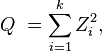
is distributed according to the chi-squared distribution with k degrees of freedom. This is usually denoted as

Q\ \sim\ \chi^2(k)\ \ \text{or}\ \ Q\ \sim\ \chi^2_k .

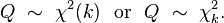
The chi-squared distribution has one parameter: k — a positive integer that specifies the number of degrees of freedom (i.e. the number of Z_i’s)

Characteristics

Further properties of the chi-squared distribution can be found in the box at the upper right corner of this article.

Probability density function

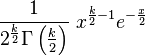
The probability density function (pdf) of the chi-squared distribution is

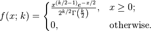
f(x;\,k) = \begin{cases} \frac{x^{(k/2-1)} e^{-x/2}}{2^{k/2} \Gamma\left(\frac{k}{2}\right)}, & x \geq 0; \\ 0, & \text{otherwise}. \end{cases}

where Γ(k/2) denotes the Gamma function, which has closed-form values for integer k.

For derivations of the pdf in the cases of one, two and k degrees of freedom, see Proofs related to chi-squared distribution.

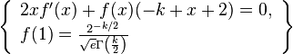
Differential equation

The pdf of the chi-squared distribution is a solution to the following differential equation:

\left\{\begin{array}{l} 2 x f'(x)+f(x) (-k+x+2)=0, \\ f(1)=\frac{2^{-k/2}}{\sqrt{e} \Gamma \left(\frac{k}{2}\right)} \end{array}\right\}

Cumulative distribution function

Chernoff bound for the CDF and tail (1-CDF) of a chi-squared random variable with ten degrees of freedom (k = 10)

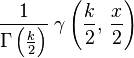
Its cumulative distribution function is:

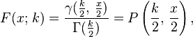
F(x;\,k) = \frac{\gamma(\frac{k}{2},\,\frac{x}{2})}{\Gamma(\frac{k}{2})} = P\left(\frac{k}{2},\,\frac{x}{2}\right),

where γ(s,t) is the lower incomplete Gamma function and P(s,t) is the regularized Gamma function.

In a special case of k = 2 this function has a simple form:

F(x;\,2) = 1 - e^{-\frac{x}{2}}

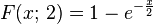
and the form is not much more complicated for other small even k.

Tables of the chi-squared cumulative distribution function are widely available and the function is included in many spreadsheets and all statistical packages.

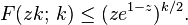
Letting $z \equiv x/k$ , Chernoff bounds on the lower and upper tails of the CDF may be obtained.^[9] For the cases when $0 < z < 1$ (which include all of the cases when this CDF is less than half):

F(z k;\,k) \leq (z e^{1-z})^{k/2}.

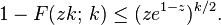
The tail bound for the cases when $z > 1$ , similarly, is

1-F(z k;\,k) \leq (z e^{1-z})^{k/2}.

For another approximation for the CDF modeled after the cube of a Gaussian, see under Noncentral chi-squared distribution.

Additivity

It follows from the definition of the chi-squared distribution that the sum of independent chi-squared variables is also chi-squared distributed. Specifically, if {X_i}_i=1ⁿ are independent chi-squared variables with {k_i}_i=1ⁿ degrees of freedom, respectively, then Y = X₁ + ⋯ + X_n is chi-squared distributed with k₁ + ⋯ + k_n degrees of freedom.

Sample mean

The sample mean of n i.i.d. chi-squared variables of degree k is distributed according to a gamma distribution with shape α and scale θ parameters: $\bar X = \frac{1}{n} \sum_{i=1}^{n} X_i \sim \mathrm{Gamma}\left(\alpha=n\, k /2, \theta= 2/n \right) \qquad \mathrm{where } \quad X_i \sim \chi^2(k)$

Asymptotically, given that for a scale parameter $\alpha$ going to infinity, a Gamma distribution converges towards a Normal distribution with expectation $\mu = \alpha\cdot \theta$ and variance $\sigma^2 = \alpha\, \theta^2$ , the sample mean converges towards: $\bar X \xrightarrow{n \to \infty} N(\mu = k, \sigma^2 = 2\, k /n )$

Note that we would have obtained the same result invoking instead the central limit theorem, noting that for each chi-squared variable of degree $k$ the expectation is $k$ , and its variance $2\,k$ (and hence the variance of the sample mean $\bar X$ being $\sigma^2 = 2\,k/n$ ).

Entropy

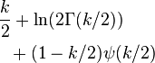
The differential entropy is given by

h = \int_{-\infty}^\infty f(x;\,k)\ln f(x;\,k) \, dx = \frac{k}{2} + \ln\!\left[2\,\Gamma\!\left(\frac{k}{2}\right)\right] + \left(1-\frac{k}{2}\right)\, \psi\!\left[\frac{k}{2}\right],

where ψ(x) is the Digamma function.

The chi-squared distribution is the maximum entropy probability distribution for a random variate X for which $E(X)=k$ and $E(\ln(X))=\psi\left(k/2\right)+log(2)$ are fixed. Since the chi-squared is in the family of gamma distributions, this can be derived by substituting appropriate values in the Expectation of the Log moment of Gamma. For derivation from more basic principles, see the derivation in moment generating function of the sufficient statistic.

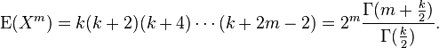
Noncentral moments

The moments about zero of a chi-squared distribution with k degrees of freedom are given by^[10]^[11]

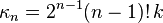
\operatorname{E}(X^m) = k (k+2) (k+4) \cdots (k+2m-2) = 2^m \frac{\Gamma(m+\frac{k}{2})}{\Gamma(\frac{k}{2})}.

Cumulants

The cumulants are readily obtained by a (formal) power series expansion of the logarithm of the characteristic function:

\kappa_n = 2^{n-1}(n-1)!\,k

Asymptotic properties

By the central limit theorem, because the chi-squared distribution is the sum of k independent random variables with finite mean and variance, it converges to a normal distribution for large k. For many practical purposes, for k > 50 the distribution is sufficiently close to a normal distribution for the difference to be ignored.^[12] Specifically, if X ~ χ²(k), then as k tends to infinity, the distribution of 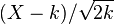$(X-k)/\sqrt{2k}$ tends to a standard normal distribution. However, convergence is slow as the skewness is $\sqrt{8/k}$ and the excess kurtosis is 12/k.

The sampling distribution of ln(χ²) converges to normality much faster than the sampling distribution of χ²,^[13] as the logarithm removes much of the asymmetry.^[14] Other functions of the chi-squared distribution converge more rapidly to a normal distribution. Some examples are:
If X ~ χ²(k) then $\scriptstyle\sqrt{2X}$ is approximately normally distributed with mean $\scriptstyle\sqrt{2k-1}$ and unit variance (result credited to R. A. Fisher).
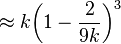
If X ~ χ²(k) then $\scriptstyle\sqrt[3]{X/k}$ is approximately normally distributed with mean $\scriptstyle 1-2/(9k)$ and variance $\scriptstyle 2/(9k) .$ ^[15] This is known as the Wilson–Hilferty transformation.

Relation to other distributions

Approximate formula for median compared with numerical quantile (top). Difference between numerical quantile and approximate formula (bottom).

As $k\to\infty$ , $(\chi^2_k-k)/\sqrt{2k} ~ \xrightarrow{d}\ N(0,1) \,$ (normal distribution)

$\chi_k^2 \sim {\chi'}^2_k(0)$ (Noncentral chi-squared distribution with non-centrality parameter $\lambda = 0$ )

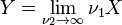If $X \sim \mathrm{F}(\nu_1, \nu_2)$ then $Y = \lim_{\nu_2 \to \infty} \nu_1 X$ has the chi-squared distribution $\chi^2_{\nu_{1}}$

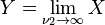As a special case, if $X \sim \mathrm{F}(1, \nu_2)\,$ then $Y = \lim_{\nu_2 \to \infty} X\,$ has the chi-squared distribution $\chi^2_{1}$

$\|\boldsymbol{N}_{i=1,...,k}{(0,1)}\|^2 \sim \chi^2_k$ (The squared norm of k standard normally distributed variables is a chi-squared distribution with k degrees of freedom)

If $X \sim {\chi}^2(\nu)\,$ and $c>0 \,$ , then $cX \sim {\Gamma}(k=\nu/2, \theta=2c)\,$ . (gamma distribution)

If $X \sim \chi^2_k$ then $\sqrt{X} \sim \chi_k$ (chi distribution)

If $X \sim \chi^2 \left( 2 \right)$ , then $X \sim \mathrm{Exp(1/2)}$ is an exponential distribution. (See Gamma distribution for more.)

If $X \sim \mathrm{Rayleigh}(1)\,$ (Rayleigh distribution) then $X^2 \sim \chi^2(2)\,$

If $X \sim \mathrm{Maxwell}(1)\,$ (Maxwell distribution) then $X^2 \sim \chi^2(3)\,$

If $X \sim \chi^2(\nu)$ then $\tfrac{1}{X} \sim \mbox{Inv-}\chi^2(\nu)\,$ (Inverse-chi-squared distribution)

The chi-squared distribution is a special case of type 3 Pearson distribution

If $X \sim \chi^2(\nu_1)\,$ and $Y \sim \chi^2(\nu_2)\,$ are independent then $\tfrac{X}{X+Y} \sim {\rm Beta}(\tfrac{\nu_1}{2}, \tfrac{\nu_2}{2})\,$ (beta distribution)

If $X \sim {\rm U}(0,1)\,$ (uniform distribution) then $-2\log{(X)} \sim \chi^2(2)\,$

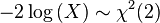
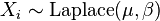
$\chi^2(6)\,$ is a transformation of Laplace distribution

If $X_i \sim \mathrm{Laplace}(\mu,\beta)\,$ then $\sum_{i=1}^n{\frac{2 |X_i-\mu|}{\beta}} \sim \chi^2(2n)\,$

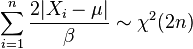
chi-squared distribution is a transformation of Pareto distribution

Student's t-distribution is a transformation of chi-squared distribution

Student's t-distribution can be obtained from chi-squared distribution and normal distribution

Noncentral beta distribution can be obtained as a transformation of chi-squared distribution and Noncentral chi-squared distribution

Noncentral t-distribution can be obtained from normal distribution and chi-squared distribution

A chi-squared variable with k degrees of freedom is defined as the sum of the squares of k independent standard normal random variables.

If Y is a k-dimensional Gaussian random vector with mean vector μ and rank k covariance matrix C, then X = (Y−μ)^TC⁻¹(Y−μ) is chi-squared distributed with k degrees of freedom.

The sum of squares of statistically independent unit-variance Gaussian variables which do not have mean zero yields a generalization of the chi-squared distribution called the noncentral chi-squared distribution.

If Y is a vector of k i.i.d. standard normal random variables and A is a k×k symmetric, idempotent matrix with rank k−n then the quadratic form Y^TAY is chi-squared distributed with k−n degrees of freedom.

The chi-squared distribution is also naturally related to other distributions arising from the Gaussian. In particular,

Y is F-distributed, Y ~ F(k₁,k₂) if $\scriptstyle Y = \frac{X_1 / k_1}{X_2 / k_2}$ where X₁ ~ χ²(k₁) and X₂ ~ χ²(k₂) are statistically independent.

If X is chi-squared distributed, then $\scriptstyle\sqrt{X}$ is chi distributed.

If X₁ ~ χ²_k₁ and X₂ ~ χ²_k₂ are statistically independent, then X₁ + X₂ ~ χ²_k₁+k₂. If X₁ and X₂ are not independent, then X₁ + X₂ is not chi-squared distributed.

Generalizations

The chi-squared distribution is obtained as the sum of the squares of k independent, zero-mean, unit-variance Gaussian random variables. Generalizations of this distribution can be obtained by summing the squares of other types of Gaussian random variables. Several such distributions are described below.

Linear combination

If $X_1,...,X_n$ are chi square random variables and $a_1,...,a_n\in\mathbb{R}_{>0}$ , then a closed expression for the distribution of 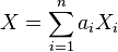$X=\sum_{i=1}^n a_iX_i$ is not known. It may be, however, calculated using the property of characteristic functions of the chi-squared random variable.^[16]

Chi-squared distributions

Noncentral chi-squared distribution

Main article: Noncentral chi-squared distribution

The noncentral chi-squared distribution is obtained from the sum of the squares of independent Gaussian random variables having unit variance and nonzero means.

Generalized chi-squared distribution

Main article: Generalized chi-squared distribution

The generalized chi-squared distribution is obtained from the quadratic form z′Az where z is a zero-mean Gaussian vector having an arbitrary covariance matrix, and A is an arbitrary matrix.

Gamma, exponential, and related distributions

The chi-squared distribution X ~ χ²(k) is a special case of the gamma distribution, in that X ~ Γ(k/2, 1/2) using the rate parameterization of the gamma distribution (or X ~ Γ(k/2, 2) using the scale parameterization of the gamma distribution) where k is an integer.

Because the exponential distribution is also a special case of the Gamma distribution, we also have that if X ~ χ²(2), then X ~ Exp(1/2) is an exponential distribution.

The Erlang distribution is also a special case of the Gamma distribution and thus we also have that if X ~ χ²(k) with even k, then X is Erlang distributed with shape parameter k/2 and scale parameter 1/2.

Applications

The chi-squared distribution has numerous applications in inferential statistics, for instance in chi-squared tests and in estimating variances. It enters the problem of estimating the mean of a normally distributed population and the problem of estimating the slope of a regression line via its role in Student’s t-distribution. It enters all analysis of variance problems via its role in the F-distribution, which is the distribution of the ratio of two independent chi-squared random variables, each divided by their respective degrees of freedom.

Following are some of the most common situations in which the chi-squared distribution arises from a Gaussian-distributed sample.

if X₁, ..., X_n are i.i.d. N(μ, σ²) random variables, then 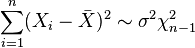$\sum_{i=1}^n(X_i - \bar X)^2 \sim \sigma^2 \chi^2_{n-1}$ where $\bar X = \frac{1}{n} \sum_{i=1}^n X_i$ .

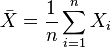The box below shows some statistics based on X_i ∼ Normal(μ_i, σ²_i), i = 1, ⋯, k, independent random variables that have probability distributions related to the chi-squared distribution:

Name	Statistic
chi-squared distribution	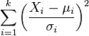$\sum_{i=1}^k \left(\frac{X_i-\mu_i}{\sigma_i}\right)^2$
noncentral chi-squared distribution	$\sum_{i=1}^k \left(\frac{X_i}{\sigma_i}\right)^2$
chi distribution	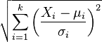$\sqrt{\sum_{i=1}^k \left(\frac{X_i-\mu_i}{\sigma_i}\right)^2}$
noncentral chi distribution	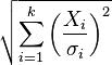$\sqrt{\sum_{i=1}^k \left(\frac{X_i}{\sigma_i}\right)^2}$

The chi-squared distribution is also often encountered in Magnetic Resonance Imaging .^[17]

Table of χ² value vs p-value

The p-value is the probability of observing a test statistic at least as extreme in a chi-squared distribution. Accordingly, since the cumulative distribution function (CDF) for the appropriate degrees of freedom (df) gives the probability of having obtained a value less extreme than this point, subtracting the CDF value from 1 gives the p-value. The table below gives a number of p-values matching to χ² for the first 10 degrees of freedom.

A low p-value indicates greater statistical significance, i.e. greater confidence that the observed deviation from the null hypothesis is significant. A p-value of 0.05 is often used as a bright-line cutoff between significant and not-significant results.

Degrees of freedom (df)	χ² value^[18]
1	0.004	0.02	0.06	0.15	0.46	1.07	1.64	2.71	3.84	6.64	10.83
2	0.10	0.21	0.45	0.71	1.39	2.41	3.22	4.60	5.99	9.21	13.82
3	0.35	0.58	1.01	1.42	2.37	3.66	4.64	6.25	7.82	11.34	16.27
4	0.71	1.06	1.65	2.20	3.36	4.88	5.99	7.78	9.49	13.28	18.47
5	1.14	1.61	2.34	3.00	4.35	6.06	7.29	9.24	11.07	15.09	20.52
6	1.63	2.20	3.07	3.83	5.35	7.23	8.56	10.64	12.59	16.81	22.46
7	2.17	2.83	3.82	4.67	6.35	8.38	9.80	12.02	14.07	18.48	24.32
8	2.73	3.49	4.59	5.53	7.34	9.52	11.03	13.36	15.51	20.09	26.12
9	3.32	4.17	5.38	6.39	8.34	10.66	12.24	14.68	16.92	21.67	27.88
10	3.94	4.87	6.18	7.27	9.34	11.78	13.44	15.99	18.31	23.21	29.59
P value (Probability)	0.95	0.90	0.80	0.70	0.50	0.30	0.20	0.10	0.05	0.01	0.001

References

↑ M.A. Sanders. "Characteristic function of the central chi-squared distribution" (PDF). Retrieved 2009-03-06.
↑ Abramowitz, Milton; Stegun, Irene A., eds. (1965), "Chapter 26", Handbook of Mathematical Functions with Formulas, Graphs, and Mathematical Tables, New York: Dover, p. 940, ISBN 978-0486612720, MR 0167642 .
↑ NIST (2006). Engineering Statistics Handbook - Chi-Squared Distribution
↑ Jonhson, N. L.; Kotz, S.; Balakrishnan, N. (1994). "Chi-Squared Distributions including Chi and Rayleigh". Continuous Univariate Distributions 1 (Second ed.). John Willey and Sons. pp. 415–493. ISBN 0-471-58495-9.
↑ Mood, Alexander; Graybill, Franklin A.; Boes, Duane C. (1974). Introduction to the Theory of Statistics (Third ed.). McGraw-Hill. pp. 241–246. ISBN 0-07-042864-6.
↑ 6.0 6.1 Hald 1998, pp. 633–692, 27. Sampling Distributions under Normality.
↑ F. R. Helmert, "Ueber die Wahrscheinlichkeit der Potenzsummen der Beobachtungsfehler und über einige damit im Zusammenhange stehende Fragen", Zeitschrift für Mathematik und Physik 21, 1876, S. 102–219
↑ R. L. Plackett, Karl Pearson and the Chi-Squared Test, International Statistical Review, 1983, 61f. See also Jeff Miller, Earliest Known Uses of Some of the Words of Mathematics.
↑ Dasgupta, Sanjoy D. A.; Gupta, Anupam K. (2002). "An Elementary Proof of a Theorem of Johnson and Lindenstrauss" (PDF). Random Structures and Algorithms 22: 60–65. doi:10.1002/rsa.10073. Retrieved 2012-05-01.
↑ Chi-squared distribution, from MathWorld, retrieved Feb. 11, 2009
↑ M. K. Simon, Probability Distributions Involving Gaussian Random Variables, New York: Springer, 2002, eq. (2.35), ISBN 978-0-387-34657-1
↑ Box, Hunter and Hunter (1978). Statistics for experimenters. Wiley. p. 118. ISBN 0471093157.
↑ Bartlett, M. S.; Kendall, D. G. (1946). "The Statistical Analysis of Variance-Heterogeneity and the Logarithmic Transformation". Supplement to the Journal of the Royal Statistical Society 8 (1): 128–138. JSTOR 2983618.
↑ Shoemaker, Lewis H. (2003). "Fixing the F Test for Equal Variances". The American Statistician 57 (2): 105–114. doi:10.1198/0003130031441. JSTOR 30037243.
↑ Wilson, E. B.; Hilferty, M. M. (1931). "The distribution of chi-squared" (PDF). Proc. Natl. Acad. Sci. USA 17 (12): 684–688.
↑ Davies, R.B. (1980). "Algorithm AS155: The Distributions of a Linear Combination of χ² Random Variables". Journal of the Royal Statistical Society 29 (3): 323–333. doi:10.2307/2346911.
↑ den Dekker A. J., Sijbers J., (2014) "Data distributions in magnetic resonance images: a review", Physica Medica,
↑ Chi-Squared Test Table B.2. Dr. Jacqueline S. McLaughlin at The Pennsylvania State University. In turn citing: R.A. Fisher and F. Yates, Statistical Tables for Biological Agricultural and Medical Research, 6th ed., Table IV

External links

Hazewinkel, Michiel, ed. (2001), "Chi-squared distribution", Encyclopedia of Mathematics, Springer, ISBN 978-1-55608-010-4
Calculator for the pdf, cdf and quantiles of the chi-squared distribution
Earliest Uses of Some of the Words of Mathematics: entry on Chi squared has a brief history
Course notes on Chi-Squared Goodness of Fit Testing from Yale University Stats 101 class.
Mathematica demonstration showing the chi-squared sampling distribution of various statistics, e.g. Σx², for a normal population
Simple algorithm for approximating cdf and inverse cdf for the chi-squared distribution with a pocket calculator

Probability distributions

Discrete univariate with finite support

Benford Bernoulli Beta-binomial binomial categorical hypergeometric Poisson binomial Rademacher discrete uniform Zipf Zipf–Mandelbrot

Discrete univariate with infinite support

beta negative binomial Borel Conway–Maxwell–Poisson discrete phase-type Delaporte extended negative binomial Gauss–Kuzmin geometric logarithmic negative binomial parabolic fractal Poisson Skellam Yule–Simon zeta

Continuous univariate supported on a bounded interval, e.g. [0,1]

Arcsine ARGUS Balding–Nichols Bates Beta Beta rectangular Irwin–Hall Kumaraswamy logit-normal Noncentral beta raised cosine Triangular U-quadratic uniform Wigner semicircle

[[List of probability distributions#Supported_on_semi-infinite_intervals.2C_usually_.5B0.2C.E2.88.9E.29|Continuous univariate supported on a semi-infinite interval, usually [0,∞)]]

Benini
Benktander 1st kind
Benktander 2nd kind
Beta prime
Burr
chi-squared
chi
Coxian
Dagum
Davis
EL
Erlang
exponential
F
folded normal
Flory-Schulz
Fréchet
Gamma
Gamma/Gompertz
generalized inverse Gaussian
Gompertz
half-logistic
half-normal
Hotelling's T-squared
hyper-Erlang
hyperexponential
hypoexponential
inverse chi-squared (scaled inverse chi-squared)
inverse Gaussian
inverse gamma
Kolmogorov
Lévy
log-Cauchy
log-Laplace
log-logistic
log-normal
matrix-exponential
Maxwell–Boltzmann
Maxwell–Jüttner
Mittag–Leffler
Nakagami
noncentral chi-squared
Pareto
phase-type
Poly-Weibull
Rayleigh
relativistic Breit–Wigner
Rice
Rosin–Rammler
shifted Gompertz
truncated normal
type-2 Gumbel
Weibull
Wilks' lambda

Continuous univariate supported on the whole real line (−∞, ∞)

Cauchy exponential power Fisher's z generalized normal generalized hyperbolic geometric stable Gumbel Holtsmark hyperbolic secant Johnson SU Landau Laplace Linnik logistic noncentral t normal (Gaussian) normal-inverse Gaussian skew normal slash stable Student's t type-1 Gumbel Tracy–Widom variance-gamma Voigt

Continuous univariate with support whose type varies

generalized extreme value generalized Pareto Tukey lambda q-Gaussian q-exponential q-Weibull shifted log-logistic

Mixed continuous-discrete univariate distributions

rectified Gaussian

Multivariate (joint)

Discrete Ewens multinomial Dirichlet-multinomial negative multinomial Continuous Dirichlet Generalized Dirichlet multivariate normal Multivariate stable multivariate Student normal-scaled inverse gamma normal-gamma Matrix-valued inverse matrix gamma inverse-Wishart matrix normal matrix t matrix gamma normal-inverse-Wishart normal-Wishart Wishart

Directional

Univariate (circular) directional Circular uniform univariate von Mises wrapped normal wrapped Cauchy wrapped exponential wrapped Lévy Bivariate (spherical) Kent Bivariate (toroidal) bivariate von Mises Multivariate von Mises–Fisher Bingham

Degenerate and singular

Degenerate discrete degenerate Dirac delta function Singular Cantor

Families

Circular compound Poisson elliptical exponential natural exponential location-scale maximum entropy mixture Pearson Tweedie wrapped

Some common univariate probability distributions

Continuous	beta Cauchy chi-squared exponential F gamma Laplace log-normal normal Pareto Student's t uniform Weibull

Discrete	Bernoulli binomial discrete uniform geometric hypergeometric negative binomial Poisson

List of probability distributions