Chernoff bound

In probability theory, the Chernoff bound, named after Herman Chernoff but due to Herman Rubin,^[1] gives exponentially decreasing bounds on tail distributions of sums of independent random variables. It is a sharper bound than the known first or second moment based tail bounds such as Markov's inequality or Chebyshev inequality, which only yield power-law bounds on tail decay. However, the Chernoff bound requires that the variates be independent – a condition that neither the Markov nor the Chebyshev inequalities require.

It is related to the (historically prior) Bernstein inequalities, and to Hoeffding's inequality.

Example

Let $X 1, ..., X n$ be independent Bernoulli random variables, each having probability p > 1/2 of being equal to 1. Then the probability of simultaneous occurrence of more than n/2 of the events ${X k = 1}$ has an exact value $S$ , where

S=\sum_{i = \lfloor \tfrac{n}{2} \rfloor + 1}^n \binom{n}{i}p^i (1 - p)^{n - i} .

The Chernoff bound shows that $S$ has the following lower bound:

S \ge 1 - e^{-\frac{1}{2p}n \left(p - \frac{1}{2} \right)^2} .

Indeed, noticing that $μ = np$ , we get by the multiplicative form of Chernoff bound (see below or Corollary 13.3 in Sinclair's class notes),^[2]

\begin{align} \Pr\left (\sum_{k=1}^n X_k \le\left\lfloor \tfrac{n}{2}\right\rfloor \right ) &=\Pr\left (\sum_{k=1}^n X_k\le\left(1-\left(1-\tfrac{1}{2p}\right)\right)\mu\right ) \\ &\leq e^{-\frac{\mu}{2}\left(1-\frac{1}{2p}\right)^2} \\ &=e^{-\frac{n}{2p}\left(p-\frac{1}{2}\right)^2} \end{align}

This result admits various generalizations as outlined below. One can encounter many flavours of Chernoff bounds: the original additive form (which gives a bound on the absolute error) or the more practical multiplicative form (which bounds the error relative to the mean).

A motivating example

The simplest case of Chernoff bounds is used to bound the success probability of majority agreement for $n$ independent, equally likely events.

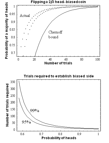
A simple motivating example is to consider a biased coin. One side (say, Heads), is more likely to come up than the other, but you don't know which and would like to find out. The obvious solution is to flip it many times and then choose the side that comes up the most. But how many times do you have to flip it to be confident that you've chosen correctly?

In our example, let $X i$ denote the event that the ith coin flip comes up Heads; suppose that we want to ensure we choose the wrong side with at most a small probability $ε$ . Then, rearranging the above, we must have:

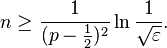
n \geq \frac{1}{(p -\frac{1}{2})^2} \ln \frac{1}{\sqrt{\varepsilon}}.

If the coin is noticeably biased, say coming up on one side 60% of the time (p = .6), then we can guess that side with 95% (ε = .05) accuracy after 150 flips (n = 150). If it is 90% biased, then a mere 10 flips suffices. If the coin is only biased a tiny amount, like most real coins are, the number of necessary flips becomes much larger.

More practically, the Chernoff bound is used in randomized algorithms (or in computational devices such as quantum computers) to determine a bound on the number of runs necessary to determine a value by majority agreement, up to a specified probability. For example, suppose an algorithm (or machine) A computes the correct value of a function f with probability p > 1/2. If we choose n satisfying the inequality above, the probability that a majority exists and is equal to the correct value is at least 1 − ε, which for small enough ε is quite reliable. If p is a constant, ε diminishes exponentially with growing n, which is what makes algorithms in the complexity class BPP efficient.

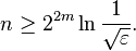
Notice that if p is very close to 1/2, the necessary $n$ can become very large. For example, if p = 1/2 + 1/2^m, as it might be in some PP algorithms, the result is that $n$ is bounded below by an exponential function in m:

n \geq 2^{2m} \ln \frac{1}{\sqrt{\varepsilon}}.

The first step in the proof of Chernoff bounds

The Chernoff bound for a random variable $X$ , which is the sum of $n$ independent random variables $X 1, ..., X n$ , is obtained by applying $e tX$ for some well-chosen value of t. This method was first applied by Sergei Bernstein to prove the related Bernstein inequalities.

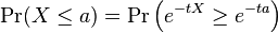
From Markov's inequality and using independence we can derive the following useful inequality:

For any t > 0,

\Pr(X \ge a) = \Pr\left (e^{tX} \ge e^{ta}\right ) \le \frac{ E \left [e^{tX} \right ]}{e^{ta}} = e^{-ta}\mathrm{E} \left [\prod_i e^{tX_i} \right].

In particular optimizing over t and using independence of $X i$ we obtain,

$\Pr(X \ge a) \leq \min_{t>0} e^{-ta} \prod_i E \left [e^{tX_i} \right ].$

(1)

Similarly,

\Pr (X \le a) = \Pr\left (e^{-tX} \ge e^{-ta}\right)

and so,

\Pr (X \le a) \leq \min_{t>0} e^{ta} \prod_i \mathrm{E} \left[e^{-tX_i} \right ]

Precise statements and proofs

Theorem for additive form (absolute error)

The following Theorem is due to Wassily Hoeffding and hence is called Chernoff-Hoeffding theorem.

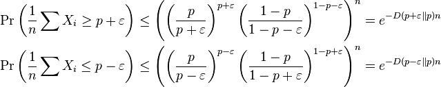
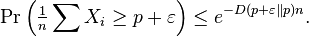
Chernoff-Hoeffding Theorem. Suppose

X 1, ..., X n

are i.i.d. random variables, taking values in

{0, 1}.

Let

p = E[X i]

and

ε > 0

. Then

\begin{align} \Pr \left (\frac{1}{n} \sum X_i \geq p + \varepsilon \right ) \leq \left (\left (\frac{p}{p + \varepsilon}\right )^{p+\varepsilon} {\left (\frac{1 - p}{1-p- \varepsilon}\right )}^{1 - p- \varepsilon}\right )^n &= e^{-D(p+\varepsilon\|p) n} \\ \Pr \left (\frac{1}{n} \sum X_i \leq p - \varepsilon \right ) \leq \left (\left (\frac{p}{p - \varepsilon}\right )^{p-\varepsilon} {\left (\frac{1 - p}{1-p+ \varepsilon}\right )}^{1 - p+ \varepsilon}\right )^n &= e^{-D(p-\varepsilon\|p) n} \end{align}

where

D(x\|y) = x \ln \frac{x}{y} + (1-x) \ln \left (\frac{1-x}{1-y} \right )

is the Kullback–Leibler divergence between Bernoulli distributed random variables with parameters x and y respectively. If

p \geq 1 / 2,

then

\Pr\left ( X>np+x \right ) \leq \exp \left (-\frac{x^2}{2np(1-p)} \right ).

Proof

Let $q = p + ε$ . Taking $a = nq$ in (1), we obtain:

\Pr\left ( \frac{1}{n} \sum X_i \ge q\right )\le \inf_{t>0} \frac{E \left[\prod e^{t X_i}\right]}{e^{tnq}} = \inf_{t>0} \left ( \frac{ E\left[e^{tX_i} \right] }{e^{tq}}\right )^n.

Now, knowing that $Pr(X i = 1) = p, Pr(X i = 0) = 1 - p$ , we have

\left (\frac{\mathrm{E}\left[e^{tX_i} \right] }{e^{tq}}\right )^n = \left (\frac{p e^t + (1-p)}{e^{tq} }\right )^n = \left ( pe^{(1-q)t} + (1-p)e^{-qt} \right )^n.

Therefore we can easily compute the infimum, using calculus:

\frac{d}{dt} \left (pe^{(1-q)t} + (1-p)e^{-qt} \right) = (1-q)pe^{(1-q)t}-q(1-p)e^{-qt}

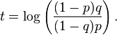
Setting the equation to zero and solving, we have

\begin{align} (1-q)pe^{(1-q)t} &= q(1-p)e^{-qt} \\ (1-q)pe^{t} &= q(1-p) \end{align}

so that

e^t = \frac{(1-p)q}{(1-q)p}.

Thus,

t = \log\left(\frac{(1-p)q}{(1-q)p}\right).

As $q = p + ε > p$ , we see that $t > 0$ , so our bound is satisfied on $t$ . Having solved for $t$ , we can plug back into the equations above to find that

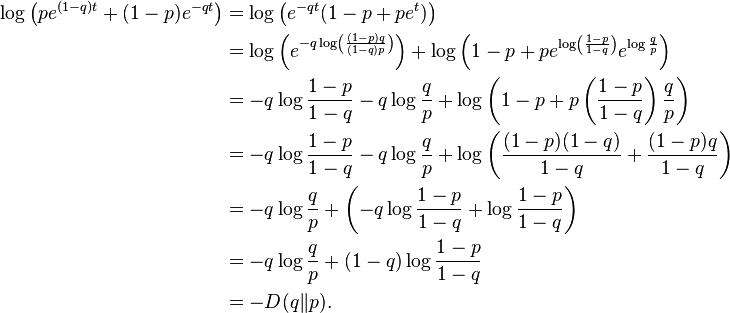
\begin{align} \log \left (pe^{(1-q)t} + (1-p)e^{-qt} \right ) &= \log \left ( e^{-qt}(1-p+pe^t) \right ) \\ &= \log\left (e^{-q \log\left(\frac{(1-p)q}{(1-q)p}\right)}\right) + \log\left(1-p+pe^{\log\left(\frac{1-p}{1-q}\right)}e^{\log\frac{q}{p}}\right ) \\ &= -q\log\frac{1-p}{1-q} -q \log\frac{q}{p} + \log\left(1-p+ p\left(\frac{1-p}{1-q}\right)\frac{q}{p}\right) \\ &= -q\log\frac{1-p}{1-q} -q \log\frac{q}{p} + \log\left(\frac{(1-p)(1-q)}{1-q}+\frac{(1-p)q}{1-q}\right) \\ &= -q \log\frac{q}{p} + \left ( -q\log\frac{1-p}{1-q} + \log\frac{1-p}{1-q} \right ) \\ &= -q\log\frac{q}{p} + (1-q)\log\frac{1-p}{1-q} \\ &= -D(q \| p). \end{align}

We now have our desired result, that

\Pr \left (\tfrac{1}{n}\sum X_i \ge p + \varepsilon\right ) \le e^{-D(p+\varepsilon\|p) n}.

To complete the proof for the symmetric case, we simply define the random variable $Y i = 1 - X i$ , apply the same proof, and plug it into our bound.

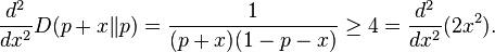
Simpler bounds

A simpler bound follows by relaxing the theorem using $D (p + x || p) \geq 2 x 2$ , which follows from the convexity of $D (p + x || p)$ and the fact that

\frac{d^2}{dx^2} D(p+x\|p) = \frac{1}{(p+x)(1-p-x)}\geq 4=\frac{d^2}{dx^2}(2x^2).

This result is a special case of Hoeffding's inequality. Sometimes, the bound

D( (1+x) p \| p) \geq \tfrac{1}{4} x^2 p, \qquad -\tfrac{1}{2} \leq x \leq \tfrac{1}{2},

which is stronger for $p < 1 / 8,$ is also used.

Theorem for multiplicative form of Chernoff bound (relative error)

Multiplicative Chernoff Bound. Suppose

X 1, ..., X n

be independent random variables taking values in

{0, 1}.

Let

X

denote their sum and let

μ = E[X]

denote the sum's expected value. For any

δ > 0

it holds that

\Pr ( X > (1+\delta)\mu) < \left(\frac{e^\delta}{(1+\delta)^{(1+\delta)}}\right)^\mu.

Proof

Set $Pr(X i = 1) = p i$ . According to (1),

\begin{align} \Pr (X > (1 + \delta)\mu) &\le \inf_{t > 0} \frac{\mathrm{E}\left[\prod_{i=1}^n\exp(tX_i)\right]}{\exp(t(1+\delta)\mu)}\\ & = \inf_{t > 0} \frac{\prod_{i=1}^n\mathrm{E}\left [e^{tX_i} \right]}{\exp(t(1+\delta)\mu)} \\ & = \inf_{t > 0} \frac{\prod_{i=1}^n\left[p_ie^t + (1-p_i)\right]}{\exp(t(1+\delta)\mu)} \end{align}

The third line above follows because $e^{tX_i}$ takes the value $e t$ with probability $p i$ and the value 1 with probability $1 - p i$ . This is identical to the calculation above in the proof of the Theorem for additive form (absolute error).

Rewriting $p_ie^t + (1-p_i)$ as $p_i(e^t-1) + 1$ and recalling that $1+x \le e^x$ (with strict inequality if $x > 0$ ), we set $x = p_i(e^t-1)$ . The same result can be obtained by directly replacing $a$ in the equation for the Chernoff bound with $(1 + δ) μ$ .^[3]

Thus,

\Pr(X > (1+\delta)\mu) < \frac{\prod_{i=1}^n\exp(p_i(e^t-1))}{\exp(t(1+\delta)\mu)} = \frac{\exp\left((e^t-1)\sum_{i=1}^n p_i\right)}{\exp(t(1+\delta)\mu)} = \frac{\exp((e^t-1)\mu)}{\exp(t(1+\delta)\mu)}.

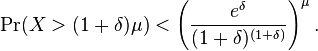
If we simply set $t = log(1 + δ)$ so that $t > 0$ for $δ > 0$ , we can substitute and find

\frac{\exp((e^t-1)\mu)}{\exp(t(1+\delta)\mu)} = \frac{\exp((1+\delta - 1)\mu)}{(1+\delta)^{(1+\delta)\mu}} = \left[\frac{e^\delta}{(1+\delta)^{(1+\delta)}}\right]^\mu

This proves the result desired. A similar proof strategy can be used to show that

\Pr(X < (1-\delta)\mu) < \left[\frac{\exp(-\delta)}{(1-\delta)^{(1-\delta)}}\right]^\mu.

The above formula is often unwieldy in practice,^[4] so the following looser but more convenient bounds are often used:

\Pr( X \ge (1+\delta)\mu) \le e^{-\frac{\delta^2\mu}{3}}, \qquad 0 < \delta < 1,

\Pr( X \le (1-\delta)\mu) \le e^{-\frac{\delta^2\mu}{2}}, \qquad 0 < \delta < 1.

Better Chernoff bounds for some special cases

We can obtain stronger bounds using simpler proof techniques for some special cases of symmetric random variables.

Suppose $X 1, ..., X n$ are independent random variables, and let $X$ denote their sum.

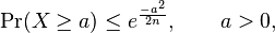
If $\Pr(X_i = 1) = \Pr(X_i = -1) = \tfrac{1}{2}$ . Then,

\Pr( X \ge a) \le e^{\frac{-a^2}{2n}}, \qquad a > 0,

and therefore also

\Pr( |X| \ge a) \le 2e^{\frac{-a^2}{2n}}, \qquad a > 0.

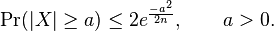
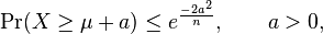
If $\Pr(X_i = 1) = \Pr(X_i = 0) = \tfrac{1}{2}, \mathrm{E}[X] = \mu = \frac{n}{2}$ Then,

\Pr( X \ge \mu+a) \le e^{\frac{-2a^2}{n}}, \qquad a > 0,

\Pr( X \le \mu-a) \le e^{\frac{-2a^2}{n}}, \qquad 0 < a < \mu,

Applications of Chernoff bound

Chernoff bounds have very useful applications in set balancing and packet routing in sparse networks.

The set balancing problem arises while designing statistical experiments. Typically while designing a statistical experiment, given the features of each participant in the experiment, we need to know how to divide the participants into 2 disjoint groups such that each feature is roughly as balanced as possible between the two groups. Refer to this book section for more info on the problem.

Chernoff bounds are also used to obtain tight bounds for permutation routing problems which reduce network congestion while routing packets in sparse networks. Refer to this book section for a thorough treatment of the problem.

Chernoff bounds can be effectively used to evaluate the "robustness level" of an application/algorithm by exploring its perturbation space with randomization. ^[5] The use of the Chernoff bound permits to abandon the strong -and mostly unrealistic- small perturbation hypothesis (the perturbation magnitude is small). The robustness level can be, in turn, used either to validate or reject a specific algorithmic choice, an hardware implementation or the appropriateness of a solution whose structural parameters are affected by uncertainties.

Matrix Chernoff bound

Main article: Matrix Chernoff bound

Rudolf Ahlswede and Andreas Winter introduced (Ahlswede & Winter 2003) a Chernoff bound for matrix-valued random variables.

If M is distributed according to some distribution over $d \times d$ matrices with zero mean, and if $M 1, ..., M t$ are independent copies of M then for any $ε > 0$ ,

\Pr\left( \left\| \frac{1}{t} \sum_{i=1}^t M_i - \mathrm{E}[M] \right\|_2 > \varepsilon \right) \leq d \exp \left( -C \frac{\varepsilon^2 t}{\gamma^2} \right).

where $\lVert M \rVert_2 \leq \gamma$ holds almost surely and C > 0 is an absolute constant.

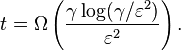
Notice that the number of samples in the inequality depends logarithmically on d. In general, unfortunately, such a dependency is inevitable: take for example a diagonal random sign matrix of dimension d. The operator norm of the sum of t independent samples is precisely the maximum deviation among d independent random walks of length t. In order to achieve a fixed bound on the maximum deviation with constant probability, it is easy to see that t should grow logarithmically with d in this scenario.^[6]

The following theorem can be obtained by assuming M has low rank, in order to avoid the dependency on the dimensions.

Theorem without the dependency on the dimensions

Let $0 < ε < 1$ and M be a random symmetric real matrix with $\| \mathrm{E}[M] \|_2 \leq 1$ and $\| M\|_2 \leq \gamma$ almost surely. Assume that each element on the support of M has at most rank r. Set

t = \Omega \left( \frac{\gamma\log (\gamma/\varepsilon^2)}{\varepsilon^2} \right).

If $r \leq t$ holds almost surely, then

\Pr\left(\left\| \frac{1}{t} \sum_{i=1}^t M_i - \mathrm{E}[M] \right\|_2 > \varepsilon \right) \leq \frac{1}{\mathbf{poly}(t)}

where $M 1, ..., M t$ are i.i.d. copies of M.

Sampling variant

The following variant of Chernoff's bound can be used to bound the probability that a majority in a population will become a minority in a sample, or vice versa.^[7]

Suppose there is a general population A and a sub-population B⊆A. Mark the relative size of the sub-population (|B|/|A|) by r.

Suppose we pick an integer k and a random sample S⊂A of size k. Mark the relative size of the sub-population in the sample (|B∩S|/|S|) by r_S.

Then, for every fraction d∈[0,1]:

\mathrm{Pr}\left(r_S < (1-d)\cdot r\right) < \exp\left(-r\cdot d^2 \cdot k/2\right)

In particular, if B is a majority in A (i.e. r > 0.5) we can bound the probability that B will remain minority in S (r_S>0.5) by taking: d = 1 - 1 / (2 r):^[8]

\mathrm{Pr}\left(r_S > 0.5\right) > 1 - \exp\left(-r\cdot \left(1 - \frac{1}{2 r}\right)^2 \cdot k/2\right)

This bound is of course not tight at all. For example, when r=0.5 we get a trivial bound Prob > 0.

References

↑ Chernoff, Herman (2014). "A career in statistics" (PDF). In Lin, Xihong; Genest, Christian; Banks, David L.; Molenberghs, Geert; Scott, David W.; Wang, Jane-Ling. Past, Present, and Future of Statistics. CRC Press. p. 35. ISBN 9781482204964.
↑ Sinclair, Alistair (Fall 2011). "Class notes for the course "Randomness and Computation"" (PDF). Retrieved 30 October 2014.
↑ Refer to the proof above
↑ Mitzenmacher, Michael and Upfal, Eli (2005). Probability and Computing: Randomized Algorithms and Probabilistic Analysis. Cambridge University Press. ISBN 0-521-83540-2.
↑ C.Alippi: "Randomized Algorithms" chapter in Intelligence for Embedded Systems. Springer, 2014, 283pp, ISBN 978-3-319-05278-6.
↑
- Magen, A.; Zouzias, A. (2011). "Low Rank Matrix-Valued Chernoff Bounds and Approximate Matrix Multiplication". arXiv:1005.2724 [cs.DM].
↑ Goldberg, A. V.; Hartline, J. D. (2001). "Competitive Auctions for Multiple Digital Goods". Algorithms — ESA 2001. Lecture Notes in Computer Science 2161. p. 416. doi:10.1007/3-540-44676-1_35. ISBN 978-3-540-42493-2. ; lemma 6.1
↑ See graphs of: the bound as a function of r when k changes and the bound as a function of k when r changes.

Chernoff, H. (1952). "A Measure of Asymptotic Efficiency for Tests of a Hypothesis Based on the sum of Observations". Annals of Mathematical Statistics 23 (4): 493–507. doi:10.1214/aoms/1177729330. JSTOR 2236576. MR 57518. Zbl 0048.11804.
Hoeffding, W. (1963). "Probability Inequalities for Sums of Bounded Random Variables". Journal of the American Statistical Association 58 (301): 13–30. doi:10.2307/2282952. JSTOR 2282952.
Chernoff, H. (1981). "A Note on an Inequality Involving the Normal Distribution". Annals of Probability 9 (3): 533. doi:10.1214/aop/1176994428. JSTOR 2243541. MR 614640. Zbl 0457.60014.
Hagerup, T. (1990). "A guided tour of Chernoff bounds". Information Processing Letters 33 (6): 305. doi:10.1016/0020-0190(90)90214-I.
Ahlswede, R.; Winter, A. (2003). "Strong Converse for Identification via Quantum Channels". IEEE Transactions on Information Theory 48 (3): 569–579. arXiv:quant-ph/0012127. doi:10.1109/18.985947.
Mitzenmacher, M.; Upfal, E. (2005). Probability and Computing: Randomized Algorithms and Probabilistic Analysis. ISBN 978-0-521-83540-4.
Nielsen, F. (2011). "Chernoff information of exponential families". arXiv:1102.2684 [cs.IT].

Chernoff bound

Example

A motivating example

The first step in the proof of Chernoff bounds

Precise statements and proofs

Theorem for additive form (absolute error)

Proof

Simpler bounds

Theorem for multiplicative form of Chernoff bound (relative error)

Proof

Better Chernoff bounds for some special cases

Applications of Chernoff bound

Matrix Chernoff bound

Theorem without the dependency on the dimensions

Sampling variant

See also

References