Characteristic equation (calculus)
In mathematics, the characteristic equation (or auxiliary equation[1]) is an algebraic equation of degree  on which depends the solutions of a given th-order differential equation.[2] The characteristic equation can only be formed when the differential equation is linear, homogeneous, and has constant coefficients.[1] Such a differential equation, with
  as the dependent variable and
  as constants,

will have a characteristic equation of the form

where  are the roots from which the general solution can be formed.[1][3][4] This method of integrating linear ordinary differential equations with constant coefficients was discovered by Leonhard Euler, who found that the solutions depended on an algebraic 'characteristic' equation.[2] The qualities of the Euler's characteristic equation were later considered in greater detail by French mathematicians Augustin-Louis Cauchy and Gaspard Monge.[2][4]
Derivation
Starting with a linear homogeneous differential equation with constant coefficients ,

it can be seen that if  , each term would be a constant multiple of
  . This results from the fact that the derivative of the exponential function is a multiple of itself. Therefore,
  ,
,  , and
, and  are all multiples. This suggests that certain values of
  will allow multiples of to sum to zero, thus solving the homogeneous differential equation.[3] In order to solve for , one can substitute
  and its derivatives into the differential equation to get

Since can never equate to zero, it can be divided out, giving the characteristic equation
By solving for the roots, , in this characteristic equation, one can find the general solution to the differential equation.[1][4] For example, if is found to equal to 3, then the general solution will be  , where
  is an arbitrary constant.
Formation of the general solution
| Example |
|---|
|
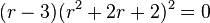
The linear homogeneous differential equation with constant coefficients has the characteristic equation By factoring the characteristic equation into one can see that the solutions for |


 and the double complex root
  . This corresponds to the real-valued general solution with constants
  of
of
Solving the characteristic equation for its roots,  , allows one to find the general solution of the differential equation. The roots may be real and/or complex, as well as distinct and/or repeated. If a characteristic equation has parts with distinct real roots,
  repeated roots, and/or
  complex roots corresponding to general solutions of
  ,
,  , and
, and  , respectively, then the general solution to the differential equation is

Distinct real roots
The superposition principle for linear homogeneous differential equations with constant coefficients says that if  are linearly independent solutions to a particular differential equation, then
  is also a solution for all values
  .[1][5] Therefore, if the characteristic equation has distinct real roots , then a general solution will be of the form

Repeated real roots
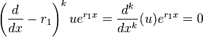
If the characteristic equation has a root  that is repeated times, then it is clear that
  is at least one solution.[1] However, this solution lacks linearly independent solutions from the other
  roots. Since has multiplicity , the differential equation can be factored into[1]
The fact that is one solution allows one to presume that the general solution may be of the form  , where
  is a function to be determined. Substituting
  gives
gives

when  . By applying this fact times, it follows that
By dividing out  , it can be seen that
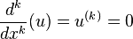
However, this is the case if and only if is a polynomial of degree , so that  .[4] Since
 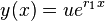 , the part of the general solution corresponding to
  is
is

Complex roots
If the characteristic equation has complex roots of the form  and
and  , then the general solution is accordingly
 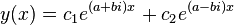 . However, by Euler's formula, which states that
 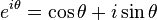 , this solution can be rewritten as follows:
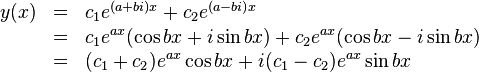
where  and
and  are constants that can be complex.[4]
Note that if  , then the particular solution
 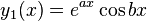 is formed.
Similarly, if  and
and  , then the independent solution formed is
 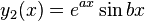 . Thus by the superposition principle for linear homogeneous differential equations with constant coefficients, the part of a differential equation having complex roots
  will result in the following general solution:
References
- ↑ 1.0 1.1 1.2 1.3 1.4 1.5 1.6 Edwards, C. Henry; Penney, David E. "3". Differential Equations: Computing and Modeling. David Calvis. Upper Saddle River, New Jersey: Pearson Education. pp. 156–170. ISBN 978-0-13-600438-7.
- ↑ 2.0 2.1 2.2 Smith, David Eugene. "History of Modern Mathematics: Differential Equations". University of South Florida.
- ↑ 3.0 3.1 Chu, Herman; Shah, Gaurav; Macall, Tom. "Linear Homogeneous Ordinary Differential Equations with Constant Coefficients". eFunda. Retrieved 1 March 2011.
- ↑ 4.0 4.1 4.2 4.3 4.4 Cohen, Abraham (1906). An Elementary Treatise on Differential Equations. D. C. Heath and Company.
- ↑ Dawkins, Paul. "Differential Equation Terminology". Paul's Online Math Notes. Retrieved 2 March 2011.