Change of variables (PDE)
Often a partial differential equation can be reduced to a simpler form with a known solution by a suitable change of variables.
The article discusses change of variable for PDEs below in two ways:
- by example;
- by giving the theory of the method.
Explanation by example
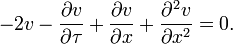
For example the following simplified form of the Black–Scholes PDE
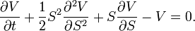
is reducible to the heat equation

by the change of variables:[1]
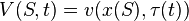
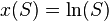
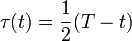

in these steps:
- Replace
 by
by 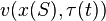 and apply the chain rule to get

- Replace
 and
and  by
by  and
and  to get

- Replace and by and and divide both sides by
 to get
- Replace
 by
by  and divide through by
  to yield the heat equation.
Advice on the application of change of variable to PDEs is given by mathematician J. Michael Steele:[2]
"There is nothing particularly difficult about changing variables and transforming one equation to another, but there is an element of tedium and complexity that slows us down. There is no universal remedy for this molasses effect, but the calculations do seem to go more quickly if one follows a well-defined plan. If we know thatdefined in terms of the old if we write the old V as a function of the new v and write the new
and x as functions of the old t and S. This order of things puts everything in the direct line of fire of the chain rule; the partial derivatives
,
and
are easy to compute and at the end, the original equation stands ready for immediate use."
Technique in general
Suppose that we have a function  and a change of variables
  such that there exist functions
 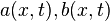 such that


and functions 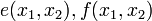 such that
and furthermore such that


and
In other words, it is helpful for there to be a bijection between the old set of variables and the new one, or else one has to
- Restrict the domain of applicability of the correspondence to a subject of the real plane which is sufficient for a solution of the practical problem at hand (where again it needs to be a bijection), and
- Enumerate the (zero or more finite list) of exceptions (poles) where the otherwise-bijection fails (and say why these exceptions don't restrict the applicability of the solution of the reduced equation to the original equation)
If a bijection does not exist then the solution to the reduced-form equation will not in general be a solution of the original equation.
We are discussing change of variable for PDEs. A PDE can be expressed as a differential operator applied to a function. Suppose  is a differential operator such that
Then it is also the case that
where

and we operate as follows to go from  to
to 
- Apply the chain rule to
 and expand out giving equation
  .
. - Substitute
 for
for  and
and  for
for  in and expand out giving equation
  .
. - Replace occurrences of
 by
by  and
and  by
by  to yield
  , which will be free of and .
Action-angle coordinates
Often, theory can establish the existence of a change of variables, although the formula itself cannot be explicitly stated. For an integrable Hamiltonian system of dimension  , with
  and
and  , there exist integrals
  . There exists a change of variables from the coordinates
  to a set of variables
  , in which the equations of motion become
  ,
, 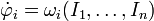 , where the functions
  are unknown, but depend only on
  . The variables are the action coordinates, the variables
  are the angle coordinates. The motion of the system can thus be visualized as rotation on torii. As a particular example, consider the simple harmonic oscillator, with
  and
and  , with Hamiltonian
 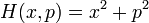 . This system can be rewritten as
  ,
,  , where
  and
and  are the canonical polar coordinates:
  and
and 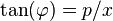 . See V. I. Arnold, `Mathematical Methods of Classical Mechanics', for more details.[3]
References
- ↑ Ömür Ugur, An Introduction to Computational Finance, Series in Quantitative Finance, v. 1, Imperial College Press, 298 pp., 2009
- ↑ J. Michael Steele, Stochastic Calculus and Financial Applications, Springer, New York, 2001
- ↑ V. I. Arnold, Mathematical Methods of Classical Mechanics, Graduate Texts in Mathematics, v. 60, Springer-Verlag, New York, 1989