Cantilever Magnetometry
Cantilever magnetometry is the use of a cantilever to measure the magnetic moment of magnetic particles. The cantilevers used for this technique are about as long as a human hair is wide (100 µm) or smaller. On the end of cantilever is glued a small piece of ferromagnetic material (called a particle), which interacts with external magnetic fields and creates torque on the cantilever. These torques cause the cantilever to oscillate faster or slower, depending on the orientation of the particle's moment with respect to the external field, and the magnitude of the moment. The magnitude of the moment and magnetic anisotropy of the particle are then deduced by measuring the cantilever's oscillation frequency while varying the external field, and finding a best fit to the resultant data.[1]

To understand this technique, it is useful to think of a pendulum: on earth it oscillates with one frequency, while if we put the same pendulum on, say, the moon, it would oscillate with a different, slower frequency. This is because the mass on the end of the pendulum interacts with the external gravitational field, much as the magnetic moment in this technique interacts with the external magnetic field. If one were to measure the frequency of a pendulum (and the length), they could extract the gravitational field since 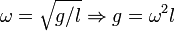 , whereas in this technique one measures the frequency and extracts the moment.
Cantilever Equation of Motion
As the cantilever oscillates back and forth it arches into hyperbolic curves with the salient feature that a tangent to the end of the cantilever always intersects one point along the middle axis. From this we define the effective length of the cantilever,  , to be the distance from this point to the end of the cantilever (see image to the right). The Lagrangian for this system is then given by
-
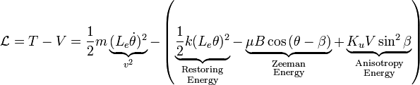
(Eq. 1)
where  is the effective cantilever mass,
  is the volume of the particle,
  is the cantilever-constant and
  is the magnetic moment of the particle. To find the equation of motion we note that we have two variables,
  and
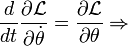
and  so there are two corresponding Lagrangian equations which need to be solved as a system of equations,
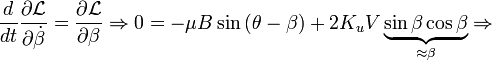
-
(Eq. 2)
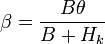
where we have defined 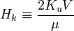 .
.
We can plug Eq. 2 into our Lagrangian, which then becomes a function of only. Then 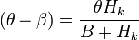 , and we have

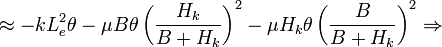
or
-
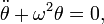
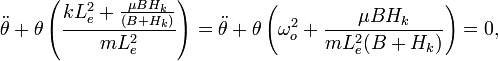
(Eq. 3)
where 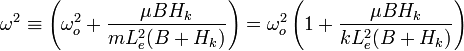 . The solution to this differential equation is
  where
where  and
and  are coefficients determined by the initial conditions. It is interesting to note that the motion of a simple pendulum is similarly described by this differential equation and solution in the small angle approximation.
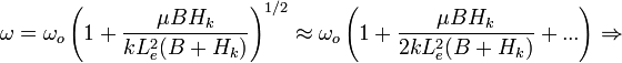
We can use the binomial expansion to rewrite  ,
,
-
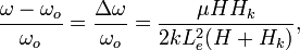
(Eq. 4)
-
which is the form as seen in literature, for example equation 2 in the paper "Magnetic Dissipation and Fluctuations in Individual Nanomagnets Measured by Ultrasensitive Cantilever Magnetometry" [1]
- ↑ 1.0 1.1 Rugar, Dan; Stipe, Mamin, Stowe, Kenny (2001). Physical Review Letters 86 (13). doi:10.1103/physrevlett.86.2874 http://phy-dhcp-35-17.mps.ohio-state.edu/HammelGroupWiki/images/6/6a/PhysRevLett.86.2874.pdf. Missing or empty
|title=(help)