Caccioppoli set
In mathematics, a Caccioppoli set is a set whose boundary is measurable and has a (at least locally) finite measure. A synonym is set of (locally) finite perimeter. Basically, a set is a Caccioppoli set if its characteristic function is a function of bounded variation.
History
The basic concept of a Caccioppoli set was firstly introduced by the Italian mathematician Renato Caccioppoli in the paper (Caccioppoli 1927): considering a plane set or a surface defined on an open set in the plane, he defined their measure or area as the total variation in the sense of Tonelli of their defining functions, i.e. of their parametric equations, provided this quantity was bounded. The measure of the boundary of a set was defined as a functional, precisely a set function, for the first time: also, being defined on open sets, it can be defined on all Borel sets and its value can be approximated by the values it takes on an increasing net of subsets. Another clearly stated (and demonstrated) property of this functional was its lower semi-continuity.
In the paper (Caccioppoli 1928), he precised by using a triangular mesh as an increasing net approximating the open domain, defining positive and negative variations whose sum is the total variation, i.e. the area functional. His inspiring point of view, as he explicitly admitted, was those of Giuseppe Peano, as expressed by the Peano-Jordan Measure: to associate to every portion of a surface an oriented plane area in a similar way as an approximating chord is associated to a curve. Also, another theme found in this theory was the extension of a functional from a subspace to the whole ambient space: the use of theorems generalizing the Hahn–Banach theorem is frequently encountered in Caccioppoli research. However, the restricted meaning of total variation in the sense of Tonelli added much complication to the formal development of the theory, and the use of a parametric description of the sets restricted its scope.
Lamberto Cesari introduced the "right" generalization of functions of bounded variation to the case of several variables only in 1936:[1] perhaps, this was one of the reasons that induced Caccioppoli to present an improved version of his theory only nearly 24 years later, in the talk (Caccioppoli 1953) at the IV UMI Congress in October 1951, followed by five notes published in the Rendiconti of the Accademia Nazionale dei Lincei. These notes were sharply criticized by Laurence Chisholm Young in the Mathematical Reviews.[2]
In 1952 Ennio de Giorgi presented his first results, developing the ideas of Caccioppoli, on the definition of the measure of boundaries of sets at the Salzburg Congress of the Austrian Mathematical Society: he obtained this results by using a smoothing operator, analogous to a mollifier, constructed from the Gaussian function, independently proving some results of Caccioppoli. Probably he was led to study this theory by his teacher and friend Mauro Picone, who had also been the teacher of Caccioppoli and was likewise his friend. De Giorgi met Caccioppoli in 1953 for the first time: during their meeting, Caccioppoli expressed a profound appreciation of his work, starting their lifelong friendship.[3] The same year he published his first paper on the topic i.e. (De Giorgi 1953): however, this paper and the closely following one did not attracted much interest from the mathematical community. It was only with the paper (De Giorgi 1954), reviewed again by Laurence Chisholm Young in the Mathematical Reviews,[4] that his approach to sets of finite perimeter became widely known and appreciated: also, in the review, Young revised his previous criticism on the work of Caccioppoli.
The last paper of De Giorgi on the theory of perimeters was published in 1958: in 1959, after the death of Caccioppoli, he started to call sets of finite perimeter "Caccioppoli sets". Two years later Herbert Federer and Wendell Fleming published their paper (Federer & Fleming 1960), changing the approach to the theory. Basically they introduced two new kind of currents, respectively normal currents and integral currents: in a subsequent series of papers and in his famous treatise,[5] Federer showed that Caccioppoli sets are normal currents of dimension  in -dimensional euclidean spaces. However, even if the theory of Caccioppoli sets can be studied within the framework of theory of currents, it is customary to study it through the "traditional" approach using functions of bounded variation, as the various sections found in a lot of important monographs in mathematics and mathematical physics testify.[6]
Formal definition
In what follows, the definition and properties of functions of bounded variation in the -dimensional setting will be used.
Caccioppoli definition
Definition 1. Let  be an open subset of
  and let
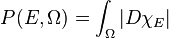
  be a Borel set. The perimeter of in is defined as follows

where  is the characteristic function of . That is, the perimeter of in an open set is defined to be the total variation of its characteristic function on that open set. If
  , then we write
  for the (global) perimeter.
Definition 2. The Borel set is a Caccioppoli set if and only if it has finite perimeter in every bounded open subset of  , i.e.
 whenever
  is open and bounded.
Therefore a Caccioppoli set has a characteristic function whose total variation is locally bounded. From the theory of functions of bounded variation it is known that this implies the existence of a vector-valued Radon measure  such that

As noted for the case of general functions of bounded variation, this vector measure is the distributional or weak gradient of . The total variation measure associated with is denoted by  , i.e. for every open set we write
  for
for  .
.
De Giorgi definition
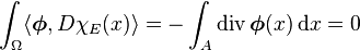
In his papers (De Giorgi 1953) and (De Giorgi 1954), Ennio de Giorgi introduces the following smoothing operator, analogous to the Weierstrass transform in the one-dimensional case

As one can easily prove,  is a smooth function for all
  , such that
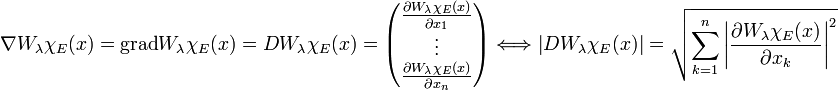
also, its gradient is everywhere well defined, and so is its absolute value
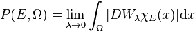
Having defined this function, De Giorgi gives the following definition of perimeter:
Definition 3. Let be an open subset of and let be a Borel set. The perimeter of in is the value
Actually De Giorgi considered the case  : however, the extension to the general case is not difficult. It can be proved that the two definitions are exactly equivalent: for a proof see the already cited De Giorgi's papers or the book (Giusti 1984). Now having defined what a perimeter is, De Giorgi gives the same definition 2 of what a set of (locally) finite perimeter is.
Basic properties
The following properties are the ordinary properties which the general notion of a perimeter is supposed to have:
- If
 then
then , with equality holding if and only if the closure of is a compact subset of .
 - For any two Cacciopoli sets
 and
and  , the relation
  holds, with equality holding if and only if
  , where
  is the distance between sets in euclidean space.
 - If the Lebesgue measure of is
 , then
  : this implies that if the symmetric difference
  of two sets has zero Lebesgue measure, the two sets have the same perimeter i.e.
  .
.
Notions of boundary
For any given Caccioppoli set  there exist two naturally associated analytic quantities: the vector-valued Radon measure and its total variation measure . Given that
is the perimeter within any open set , one should expect that alone should somehow account for the perimeter of .
The topological boundary
It is natural to try to understand the relationship between the objects , , and the topological boundary  . There is an elementary lemma that guarantees that the support (in the sense of distributions) of , and therefore also , is always contained in :
Lemma. The support of the vector-valued Radon measure is a subset of the topological boundary of .
Proof. To see this choose  : then
  belongs to the open set
  and this implies that it belongs to an open neighborhood
  contained in the interior of or in the interior of
  . Let
. Let 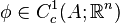 . If
. If  where
where  is the closure of , then
  for
for  and
and
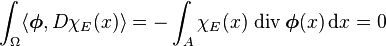
Likewise, if  then
then  for so
With  arbitrary it follows that is outside the support of .
The reduced boundary
The topological boundary turns out to be too crude for Caccioppoli sets because its Hausdorff measure overcompensates for the perimeter  defined above. Indeed, the Caccioppoli set

representing a square together with a line segment sticking out on the left has perimeter  , i.e. the extraneous line segment is ignored, while its topological boundary

has one-dimensional Hausdorff measure  .
.
The "correct" boundary should therefore be a subset of . We define:
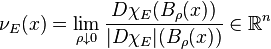
Definition 4. The reduced boundary of a Caccioppoli set is denoted by  and is defined to be equal to be the collection of points
  at which the limit:
exists and has length equal to one, i.e.  .
.
One can remark that by the Radon-Nikodym Theorem the reduced boundary is necessarily contained in the support of , which in turn is contained in the topological boundary as explained in the section above. That is:

The inclusions above are not necessarily equalities. The inclusion on the right is strict as the example of a square with a line segment sticking out shows. The inclusion on the left is strict if one considers the same square with countably many line segments sticking out densely.
De Giorgi's theorem
For convenience, in this section we treat only the case where , i.e. the set has (globally) finite perimeter. De Giorgi's theorem provides geometric intuition for the notion of reduced boundaries and confirms that it is the more natural definition for Caccioppoli sets by showing

i.e. that its Hausdorff measure equals the perimeter of the set. The statement of the theorem is quite long because it interrelates various geometric notions in one fell swoop.
Theorem. Suppose is a Caccioppoli set. Then at each point of the reduced boundary there exists a multiplicity one approximate tangent space  of , i.e. a codimension-1 subspace of such that
for every continuous, compactly supported  . In fact the subspace is the orthogonal complement of the unit vector
defined previously. This unit vector also satisfies

locally in  , so it is interpreted as an approximate inward pointing unit normal vector to the reduced boundary . Finally, is (n-1)-rectifiable and the restriction of (n-1)-dimensional Hausdorff measure
  to is , i.e.
 for all Borel sets
  .
.
In other words, up to -measure zero the reduced boundary is the smallest set on which is supported.
Applications
A Gauss–Green formula
From the definition of the vector Radon measure and from the properties of the perimeter, the following formula holds true:
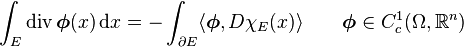
This is one version of the divergence theorem for domains with non smooth boundary. De Giorgi's theorem can be used to formulate the same identity in terms of the reduced boundary and the approximate inward pointing unit normal vector  . Precisely, the following equality holds

See also
Notes
- ↑ In the paper (Cesari 1936). See the entries "Bounded variation" and "Total variation" for more details.
- ↑ See MR MR56067.
- ↑ It lasted up to the tragic death of Caccioppoli in 1959.
- ↑ See MR 0062214.
- ↑ See (Federer 1969).
- ↑ See the "References" section.
Historical references
- Ambrosio, Luigi (2010), "La teoria dei perimetri di Caccioppoli–De Giorgi e i suoi più recenti sviluppi", Rendiconti Lincei - Matematica e Applicazioni, 9 21 (3): 275–286, doi:10.4171/RLM/572, MR 2677605, Zbl 1195.49052. "The De Giorgi-Caccioppoli theory of perimeters and its most recent developments": a paper surveying the history of the theory of sets of finite perimeter, from the seminal paper of Renato Caccioppoli and the contributions of Ennio De Giorgi to some more recent developments and open problems in metric measure spaces, in Carnot groups and in infinite-dimensional Gaussian spaces.
- Caccioppoli, Renato (1927), "Sulla quadratura delle superfici piane e curve", Atti della Accademia Nazionale dei Lincei. Rendiconti. Classe di Scienze Fisiche, Matematiche e Naturali, VI (in Italian) 6: 142–146, JFM 53.0214.02. "On the quadrature of plane and curved surfaces" is the first paper containing the seminal concept of what a Caccioppoli set is.
- Caccioppoli, Renato (1928), "Sulle coppie di funzioni a variazione limitata", Rendiconti dell'Accademia di Scienze Fisiche e Matematiche di Napoli, 3 (in Italian) 34: 83–88, JFM 54.0290.04. "On the couples of functions of bounded variation" (English translation of title) is the work where Caccioppoli made rigorous and developed the concepts introduced in the preceding paper.
- Caccioppoli, Renato (1953), "Elementi di una teoria generale dell’integrazione
 -dimensionale in uno spazio -dimensionale (Elements of a general theory of -dimensional integration in a -dimensional space)", Atti IV Congresso U.M.I., Taormina, October 1951 (in Italian) 2, Roma: Edizioni Cremonese (distributed by Unione Matematica Italiana), pp. 41–49, MR 0056067, Zbl 0051.29402.The first paper detailing the theory of finite perimeter set in a fairly complete setting.
 - Caccioppoli, Renato (1963), Opere scelte (Selected Papers), Roma: Edizioni Cremonese (distributed by Unione Matematica Italiana), pp. XXX+434 (vol. 1), 350 (vol. 2), ISBN 88-7083-505-7, Zbl 0112.28201. A selection from Caccioppoli's scientific works with a biography and a commentary of Mauro Picone.
- Cesari, Lamberto (1936), "Sulle funzioni a variazione limitata", Annali della Scuola Normale Superiore, Serie II, (in Italian) 5 (3–4): 299–313, MR 1556778, Zbl 0014.29605. Available at Numdam. Cesari's paper "On the functions of bounded variation" (English translation of the title), where he extends the now called Tonelli plane variation concept to include in the definition a subclass of the class of integrable functions.
- De Giorgi, Ennio (1953), "Definizione ed espressione analitica del perimetro di un insieme (Definition and analytical expression of the perimeter of a set)", Atti della Accademia Nazionale dei Lincei. Rendiconti. Classe di Scienze Fisiche, Matematiche e Naturali, VIII (in Italian) 14: 390–393, MR 0056066, Zbl 0051.29403. The first note published by De Giorgi describing his approach to Caccioppoli sets.
- De Giorgi, Ennio (1954),
 , Annali di Matematica Pura e Applicata, Serie IV, (in Italian) 36 (1): 191–213, doi:10.1007/BF02412838, MR 0062214, Zbl 0055.28504. The first complete exposition by De Giorgi of the theory of Caccioppoli sets.
 - Federer, Herbert; Fleming, Wendell H. (1960), "Normal and integral currents", Annals of Mathematics, Series II, 72 (4): 458–520, doi:10.2307/1970227, JSTOR 1970227, MR 0123260, Zbl 0187.31301. The first paper of Herbert Federer illustrating his approach to the theory of perimeters based on the theory of currents.
- Miranda, Mario (2003), "Caccioppoli sets", Atti della Accademia Nazionale dei Lincei, Rendiconti Lincei, Matematica e Applicazioni, IX 14 (3): 173–177, MR 2064264, Zbl 1072.49030. A paper sketching the history of the theory of sets of finite perimeter, from the seminal paper of Renato Caccioppoli to main discoveries.
References
- De Giorgi, Ennio; Colombini, Ferruccio; Piccinini, Livio (1972), Frontiere orientate di misura minima e questioni collegate, Quaderni (in Italian), Pisa: Edizioni della Normale, p. 180, MR 493669, Zbl 0296.49031. An advanced text, oriented to the theory of minimal surfaces in the multi-dimensional setting, written by one of the leading contributors. English translation of the title: "Oriented boundaries of minimal measure and related questions".
- Federer, Herbert (1996) [1969], Geometric measure theory, Classics in Mathematics, Berlin-Heidelberg-New York: Springer-Verlag New York Inc., pp. xiv+676, ISBN 3-540-60656-4, MR 0257325, Zbl 0176.00801, particularly chapter 4, paragraph 4.5, sections 4.5.1 to 4.5.4 "Sets with locally finite perimeter". The absolute reference text in geometric measure theory.
- Simon, Leon (1983), Lectures on Geometric Measure Theory, Proceedings of the Centre for Mathematical Analysis 3, Australian National University, particularly Chapter 3, Section 14 "Sets of Locally Finite Perimeter".
- Giusti, Enrico (1984), Minimal surfaces and functions of bounded variations, Monographs in Mathematics 80, Basel-Boston-Stuttgart: Birkhäuser Verlag, pp. xii+240, ISBN 0-8176-3153-4, MR 0775682, Zbl 0545.49018, particularly part I, chapter 1 "Functions of bounded variation and Caccioppoli sets". A good reference on the theory of Caccioppoli sets and their application to the Minimal surface problem.
- Hudjaev, Sergei Ivanovich; Vol'pert, Aizik Isaakovich (1985), Analysis in classes of discontinuous functions and equations of mathematical physics, Mechanics: analysis 8, Dordrecht-Boston-Lancaster: Martinus Nijhoff Publishers, pp. xviii+678, ISBN 90-247-3109-7, MR 0785938, Zbl 0564.46025, particularly part II, chapter 4 paragraph 2 "Sets with finite perimeter". One of the best books about BV-functions and their application to problems of mathematical physics, particularly chemical kinetics.
- Maz'ya, Vladimir G. (1985), Sobolev Spaces, Berlin-Heidelberg-New York: Springer-Verlag, pp. xix+486, ISBN 3-540-13589-8, MR 817985, Zbl 0692.46023; particularly chapter 6, "On functions in the space
 ". One of the best monographs on the theory of Sobolev spaces.
 - Vol'pert, Aizik Isaakovich (1967), "Spaces BV and quasi-linear equations", Matematicheskii Sbornik, (N.S.), (in Russian), 73(115) (2): 255–302, MR 216338, Zbl 0168.07402. A seminal paper where Caccioppoli sets and BV functions are deeply studied and the concept of functional superposition is introduced and applied to the theory of partial differential equations.
External links
- O'Neil, Toby Christopher (2001), "Geometric measure theory", in Hazewinkel, Michiel, Encyclopedia of Mathematics, Springer, ISBN 978-1-55608-010-4
- Zagaller, Victor Abramovich (2001), "Perimeter", in Hazewinkel, Michiel, Encyclopedia of Mathematics, Springer, ISBN 978-1-55608-010-4
- Function of bounded variation at Encyclopedia of Mathematics