Blasius boundary layer
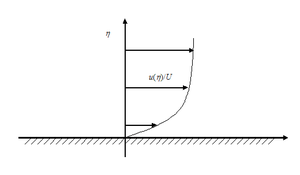
In physics and fluid mechanics, a Blasius boundary layer (named after Paul Richard Heinrich Blasius) describes the steady two-dimensional laminar boundary layer that forms on a semi-infinite plate which is held parallel to a constant unidirectional flow  .
.
 is shown, as a function of the stretched co-ordinate
  .
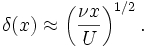
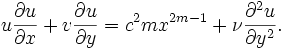
.The solution to the Navier–Stokes equation for this flow begins with an order-of-magnitude analysis to determine what terms are important. Within the boundary layer the usual balance between viscosity and convective inertia is struck, resulting in the scaling argument
 ,
,
where  is the boundary-layer thickness and
  is the kinematic viscosity.
However the semi-infinite plate has no natural length scale  and so the steady, incompressible, two-dimensional boundary-layer equations for continuity and momentum are
Continuity: 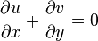
x-Momentum: 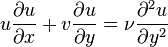
(note that the x-independence of has been accounted for in the boundary-layer equations)
admit a similarity solution. In the system of partial differential equations written above it is assumed that a fixed solid body wall is parallel to the x-direction
whereas the y-direction is normal with respect to the fixed wall, as shown in the above schematic.  and
and  denote here the x- and y-components of the fluid velocity vector.
Furthermore, from the scaling argument it is apparent that the boundary layer grows with the downstream coordinate
denote here the x- and y-components of the fluid velocity vector.
Furthermore, from the scaling argument it is apparent that the boundary layer grows with the downstream coordinate  , e.g.
This suggests adopting the similarity variable
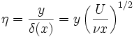
and writing

It proves convenient to work with the stream function  , in which case
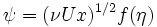
and on differentiating, to find the velocities, and substituting into the boundary-layer equation we obtain the Blasius equation
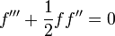
subject to
 on
on  and
and
 as
as  . This non-linear ODE can be solved numerically, with the shooting method proving an effective choice.
The shear stress on the plate
. This non-linear ODE can be solved numerically, with the shooting method proving an effective choice.
The shear stress on the plate
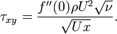
can then be computed. The numerical solution gives  .
.
Falkner–Skan boundary layer
We can generalize the Blasius boundary layer by considering a wedge at an angle of attack  from some uniform velocity field
  . We then estimate the outer flow to be of the form:
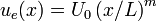
Where is a characteristic length and m is a dimensionless constant. In the Blasius solution, m = 0 corresponding to an angle of attack of zero radians. Thus we can write:

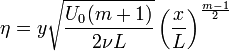
As in the Blasius solution, we use a similarity variable  to solve the Navier-Stokes Equations.
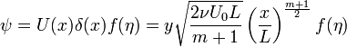
It becomes easier to describe this in terms of its stream function which we write as
Thus the initial differential equation which was written as follows:
Can now be expressed in terms of the non-linear ODE known as the Falkner–Skan equation (named after V. M. Falkner and Sylvia W. Skan[1]).
![\frac{\partial^3 f}{\partial \eta ^3}+f\frac{\partial^2 f}{\partial \eta^2}+ \beta \left[1-\left(\frac{\mathrm{d}f}{\mathrm{d}\eta}\right)^2 \right]=0](../I/m/7b3de2164863c6c977662b0bbb743604.png)
(note that  produces the Blasius equation). See Wilcox 2007.
In 1937 Douglas Hartree revealed that physical solutions exist only in the range  . Here, m < 0 corresponds to an adverse pressure gradient (often resulting in boundary layer separation) while m > 0 represents a favorable pressure gradient.
References
- ↑ V. M. Falkner and S. W. Skan, Aero. Res. Coun. Rep. and Mem. no 1314, 1930.
- Blasius, H. (1908). "Grenzschichten in Flüssigkeiten mit kleiner Reibung". Z. Math. Phys. 56: 1–37. (English translation)
- Parlange, J. Y.; Braddock, R. D.; Sander, G. (1981). "Analytical approximations to the solution of the Blasius equation". Acta Mech. 38: 119–125. doi:10.1007/BF01351467.
- Pozrikidis, C. (1998). Introduction to Theoretical and Computational Fluid Dynamics. Oxford. ISBN 0-19-509320-8.
- Lien-Tsai, Yu; Cha'o-Kuang, Chen (1998). "The solution of the blasius equation by the differential transformation method". Math. Comp. Model. 28: 101–111. doi:10.1016/S0895-7177(98)00085-5.
- He, Jihuan (1998). "Approximate analytical solution of Blasius' equation". Commun. Nonl. Sci. Num. Simul. 3 (4): 260–263. Bibcode:1998CNSNS...3..260H. doi:10.1016/S1007-5704(98)90046-6.
- Liao, S.J. (1999). "An explicit, totally analytic approximation of Blasius’ viscous flow problems". International Journal of Non-Linear Mechanics 34 (4): 759–778. Bibcode:1999IJNLM..34..759L. doi:10.1016/S0020-7462(98)00056-0. (see homotopy analysis method)
- Ropman-Miller, Lance; Broadbridge, Philip (2000). "Exact integration of reduced Fisher's equation, Reduced Balsisu equation and the Lorenz model". J. Math. An. Applic. 251 (1): 65–83. doi:10.1006/jmaa.2000.7020.
- He, Ji-Huan (2002). "A simple perturbation approach to Blasius equation". Appl. Math. Comput. 140 (2-3): 217–222. doi:10.1016/S0096-3003(02)00189-3.
- Liao, S.J.; Campo, A. (2002). "Analytic solutions of the temperature distribution in Blasius viscous flow problems". Journal of Fluid Mechanics 453: 411–425. Bibcode:2002JFM...453..411L. doi:10.1017/s0022112001007169. (see homotopy analysis method)
- Schlichting, H. (2004). Boundary-Layer Theory. Springer. ISBN 3-540-66270-7.
- Wang, Lei (2004). "A new algorithm for solving classical Blasius equation". Appl. Math. Comput. 157 (1): 1–9. doi:10.1016/j.amc.2003.06.011.
- Wilcox, David C. Basic Fluid Mechanics. DCW Industries Inc. 2007
- Abbasbandy, S. (2007). "A numerical solution of Blasius equation by Adomina's decomposition method and comparison with homotopy perturbation method". Chaos. Solit. Fract. 31 (1): 257–260. Bibcode:2007CSF....31..257A. doi:10.1016/j.chaos.2005.10.071.
- Parand, K; Deghan, Mehdi; Pirkhedri, A. (2009). "Sinc-collocation method for solving the Blasius equation". Phys. Lett. A 373 (44). Bibcode:2009PhLA..373.4060P. doi:10.1016/j.physleta.2009.09.005.
- Parand, K.; Taghavi, A. (2009). "Rational scaled generalized Laguerre function collocation method for solving the Blasius equation". J. Comp. Appl. Math. 233: 980–989. Bibcode:2009JCoAM.233..980P. doi:10.1016/j.cam.2009.08.106.