Bipartite network projection

Bipartite network projection is an extensively used method for compressing information about bipartite networks.^[1] Since the one-mode projection is always less informative than the original bipartite graph, an appropriate method for weighting network connections is often required. Optimal weighting methods reflect the nature of the specific network, conform to the designer's objectives and aim at minimizing information loss.

Background

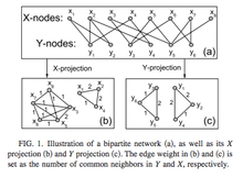
Bipartite networks are a particular class of complex networks, whose nodes are divided into two sets X and Y, and only connections between two nodes in different sets are allowed. For the convenience of directly showing the relation structure among a particular set of nodes, bipartite networks are usually compressed by one-mode projection. This means that the ensuing network contains nodes of only either of the two sets, and two X (or, alternatively, Y) nodes are connected only if when they have at least one common neighboring Y (or, alternatively, X) node.

"Possible projections of a simple bipartite network"

The simplest method involves projecting the bipartite network onto an unweighted network, without taking into account the topology of the network or the frequency of sharing a connection to the elements of the opposing set. Since bipartite networks with largely different structures can have exactly the same one-mode representation in this case, a lucid illustration of the original network topology usually requires the use of some weighting method.

Possible weighting methods

According to the designer's needs and the topological properties of the given network, several different weighting methods have been proposed. Since the redistribution of weights is found to have a strong effect on the community structure (especially in dense networks), the methodological choice must be made with care.^[2]

1. Simple weighting. Simple weighting means that edges are weighted directly by the number of times the common association is repeated. (This is the method applied in the attached graph on the right.) This approach works fine for a wide range of settings such as molecular gastronomy or most social networks. However, it can be misleading if the marginal impact of one additional association is not fixed but dependent on some characteristics of the network (e.g. on the original weight between the respective nodes). This can be the case for example in scientific collaborations as pointed out by Fan et al.^[2]
2. Hyperbolic weighting. In the common case of decreasing marginal contribution of additional links to a node, the use of simple weighting might not be very illuminating. For example, in scientific collaboration networks, two scientists whose names appear on a paper together with many other coauthors are expected to know one another less than two who were the sole authors of a paper.^[3] In order to account for this so-called saturation effect, it has been proposed to weight edges inversely according to the number of common affiliations in the neighboring set. This is most easily achieved by introducing a scaling factor 1/(n - 1) onto the simple count, which weakens the link between nodes with more popular common matches.
3. Weighting based on resource allocation. With simple and hyperbolic weighting, the projected adjacency matrix is always set to be symmetrical, which implies that a link between two projected nodes carries the same weight for both vertices. Moreover, information contained by edges whose "target" nodes are of degree 1 in the original network will be lost in the projection, which can have grievous consequences in some real networks with a lot of independent edge sets. To overcome these shortcomings, Zhou et al. has proposed a weighting method that is based on assuming that a certain amount of resource is associated with each node in the projection, and the directional weight w_ij represents the proportion of the resource node j would like to distribute to node i. Resource allocation is based on the bipartite graph, involves equal distribution across neighbors and consists of two steps: first from the projected set to the non-projected set, and then back. Numerical simulations indicate that this projecting method can perform remarkably than some widely used method (such as collaborative filtering) for personal recommendation purposes.^[1]

Some notable applications

• Flavor network and the principles of food pairing^[4]
• Scientific collaboration network ^[5]
• Corporate elite network ^[6]
• Human disease network ^[7]

References

- ↑ 1.0 1.1 "Bipartite network projection and personal recommendation" by Tao Zhou, Jie Ren, Matúš Medo and Yi-Cheng Zhang in PHYSICAL REVIEW E 76(4): 046115 (2007)
- ↑ 2.0 2.1 "The effect of weight on community structure of networks" by Ying Fan, Menghui Li, Peng Zhang, Jinshan Wu, Zengru Di in PHYSICA A 378 (2007) 583–590
- ↑ "Scientific collaboration networks. II. Shortest paths, weighted networks, and centrality" by M. E. J. Newman in PHYSICAL REVIEW E, vol. 64, 016132 (2001)