Binomial inverse theorem

In mathematics, the Binomial Inverse Theorem is useful for expressing matrix inverses in different ways.

If A, U, B, V are matrices of sizes p×p, p×q, q×q, q×p, respectively, then

provided A and B + BVA⁻¹UB are nonsingular. Note that if B is invertible, the two B terms flanking the quantity inverse in the right-hand side can be replaced with (B⁻¹)⁻¹, which results in

This is the matrix inversion lemma, which can also be derived using matrix blockwise inversion.

Verification

First notice that

Now multiply the matrix we wish to invert by its alleged inverse

which verifies that it is the inverse.

So we get that—if A⁻¹ and 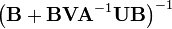exist, then exists and is given by the theorem above.^[1]

Special cases

If p = q and U = V = I_p is the identity matrix, then

Remembering the identity

we can also express the previous equation in the simpler form as

If B = I_q is the identity matrix and q = 1, then U is a column vector, written u, and V is a row vector, written v^T. Then the theorem implies

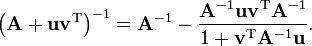
This is useful if one has a matrix with a known inverse A⁻¹ and one needs to invert matrices of the form A+uv^T quickly.

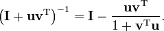
If we set A = I_p and B = I_q, we get

In particular, if q = 1, then

See also

• Woodbury matrix identity
• Sherman-Morrison formula
• Invertible matrix
• Matrix determinant lemma
• For certain cases where A is singular and also Moore-Penrose pseudoinverse, see Kurt S. Riedel, A Sherman—Morrison—Woodbury Identity for Rank Augmenting Matrices with Application to Centering, SIAM Journal on Matrix Analysis and Applications, 13 (1992)659-662, doi:10.1137/0613040 preprint MR 1152773
• Moore-Penrose pseudoinverse#Updating the pseudoinverse

References

1. ↑ Gilbert Strang (2003). Introduction to Linear Algebra (3rd edition ed.). Wellesley-Cambridge Press: Wellesley, MA. ISBN 0-9614088-9-8.