Binary decision diagram
In computer science, a binary decision diagram (BDD) or branching program, like a negation normal form (NNF) or a propositional directed acyclic graph (PDAG), is a data structure that is used to represent a Boolean function. On a more abstract level, BDDs can be considered as a compressed representation of sets or relations. Unlike other compressed representations, operations are performed directly on the compressed representation, i.e. without decompression.
Definition
A Boolean function can be represented as a rooted, directed, acyclic graph, which consists of several decision nodes and terminal nodes. There are two types of terminal nodes called 0-terminal and 1-terminal. Each decision node  is labeled by Boolean variable
  and has two child nodes called low child and high child. The edge from node
  to a low (or high) child represents an assignment of
  to 0 (resp. 1).
Such a BDD is called 'ordered' if different variables appear in the same order on all paths from the root. A BDD is said to be 'reduced' if the following two rules have been applied to its graph:
- Merge any isomorphic subgraphs.
- Eliminate any node whose two children are isomorphic.
In popular usage, the term BDD almost always refers to Reduced Ordered Binary Decision Diagram (ROBDD in the literature, used when the ordering and reduction aspects need to be emphasized). The advantage of an ROBDD is that it is canonical (unique) for a particular function and variable order.[1] This property makes it useful in functional equivalence checking and other operations like functional technology mapping.
A path from the root node to the 1-terminal represents a (possibly partial) variable assignment for which the represented Boolean function is true. As the path descends to a low (or high) child from a node, then that node's variable is assigned to 0 (resp. 1).
Example
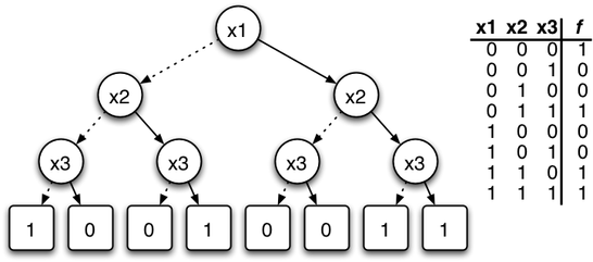
The left figure below shows a binary decision tree (the reduction rules are not applied), and a truth table, each representing the function f (x1, x2, x3). In the tree on the left, the value of the function can be determined for a given variable assignment by following a path down the graph to a terminal. In the figures below, dotted lines represent edges to a low child, while solid lines represent edges to a high child. Therefore, to find (x1=0, x2=1, x3=1), begin at x1, traverse down the dotted line to x2 (since x1 has an assignment to 0), then down two solid lines (since x2 and x3 each have an assignment to one). This leads to the terminal 1, which is the value of f (x1=0, x2=1, x3=1).
The binary decision tree of the left figure can be transformed into a binary decision diagram by maximally reducing it according to the two reduction rules. The resulting BDD is shown in the right figure.
 Binary decision tree and truth table for the function  |
 BDD for the function f |
History
The basic idea from which the data structure was created is the Shannon expansion. A switching function is split into two sub-functions (cofactors) by assigning one variable (cf. if-then-else normal form). If such a sub-function is considered as a sub-tree, it can be represented by a binary decision tree. Binary decision diagrams (BDD) were introduced by Lee,[2] and further studied and made known by Akers[3] and Boute.[4]
The full potential for efficient algorithms based on the data structure was investigated by Randal Bryant at Carnegie Mellon University: his key extensions were to use a fixed variable ordering (for canonical representation) and shared sub-graphs (for compression). Applying these two concepts results in an efficient data structure and algorithms for the representation of sets and relations.[5][6] By extending the sharing to several BDDs, i.e. one sub-graph is used by several BDDs, the data structure Shared Reduced Ordered Binary Decision Diagram is defined.[7] The notion of a BDD is now generally used to refer to that particular data structure.
In his video lecture Fun With Binary Decision Diagrams (BDDs),[8] Donald Knuth calls BDDs "one of the only really fundamental data structures that came out in the last twenty-five years" and mentions that Bryant's 1986 paper was for some time one of the most-cited papers in computer science.
Adnan Darwiche and his collaborators have shown that BDDs are one of several normal forms for Boolean functions, each induced by a different combination of requirements. Another important normal form identified by Darwiche is Decomposable Negation Normal Form or DNNF.
Applications
BDDs are extensively used in CAD software to synthesize circuits (logic synthesis) and in formal verification. There are several lesser known applications of BDD, including fault tree analysis, Bayesian reasoning, product configuration, and private information retrieval [9] [10].
Every arbitrary BDD (even if it is not reduced or ordered) can be directly implemented in hardware by replacing each node with a 2 to 1 multiplexer; each multiplexer can be directly implemented by a 4-LUT in a FPGA. It is not so simple to convert from an arbitrary network of logic gates to a BDD (unlike the and-inverter graph).
Variable ordering
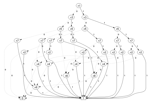
The size of the BDD is determined both by the function being represented and the chosen ordering of the variables. There exist Boolean functions  for which depending upon the ordering of the variables we would end up getting a graph whose number of nodes would be linear (in n) at the best and exponential at the worst case (e.g., a ripple carry adder). Let us consider the Boolean function
  Using the variable ordering
  , the BDD needs 2n+1 nodes to represent the function. Using the ordering
  , the BDD consists of 2n + 2 nodes.
 BDD for the function ƒ(x1, ..., x8) = x1x2 + x3x4 + x5x6 + x7x8 using bad variable ordering |
 Good variable ordering |
It is of crucial importance to care about variable ordering when applying this data structure in practice. The problem of finding the best variable ordering is NP-hard.[11] For any constant c > 1 it is even NP-hard to compute a variable ordering resulting in an OBDD with a size that is at most c times larger than an optimal one.[12] However there exist efficient heuristics to tackle the problem.[13]
There are functions for which the graph size is always exponential — independent of variable ordering. This holds e. g. for the multiplication function (an indication as to the apparent complexity of factorization ).
Researchers have of late suggested refinements on the BDD data structure giving way to a number of related graphs, such as BMD (binary moment diagrams), ZDD (zero-suppressed decision diagram), FDD (free binary decision diagrams), PDD (parity decision diagrams), and MTBDDs (multiple terminal BDDs).
Logical operations on BDDs
Many logical operations on BDDs can be implemented by polynomial-time graph manipulation algorithms.
- conjunction
- disjunction
- negation
- existential abstraction
- universal abstraction
However, repeating these operations several times, for example forming the conjunction or disjunction of a set of BDDs, may in the worst case result in an exponentially big BDD. This is because any of the preceding operations for two BDDs may result in a BDD with a size proportional to the product of the BDDs' sizes, and consequently for several BDDs the size may be exponential.
See also
- Boolean satisfiability problem
- L/poly, a complexity class that captures the complexity of problems with polynomially sized BDDs
- Model checking
- Radix tree
- Binary key – a method of species identification in biology using binary trees
- Barrington's theorem
References
- ↑ Graph-Based Algorithms for Boolean Function Manipulation, Randal E. Bryant, 1986
- ↑ C. Y. Lee. "Representation of Switching Circuits by Binary-Decision Programs". Bell Systems Technical Journal, 38:985–999, 1959.
- ↑ Sheldon B. Akers. Binary Decision Diagrams, IEEE Transactions on Computers, C-27(6):509–516, June 1978.
- ↑ Raymond T. Boute, "The Binary Decision Machine as a programmable controller". EUROMICRO Newsletter, Vol. 1(2):16–22, January 1976.
- ↑ Randal E. Bryant. "Graph-Based Algorithms for Boolean Function Manipulation". IEEE Transactions on Computers, C-35(8):677–691, 1986.
- ↑ R. E. Bryant, "Symbolic Boolean Manipulation with Ordered Binary Decision Diagrams", ACM Computing Surveys, Vol. 24, No. 3 (September, 1992), pp. 293–318.
- ↑ Karl S. Brace, Richard L. Rudell and Randal E. Bryant. "Efficient Implementation of a BDD Package". In Proceedings of the 27th ACM/IEEE Design Automation Conference (DAC 1990), pages 40–45. IEEE Computer Society Press, 1990.
- ↑ http://scpd.stanford.edu/knuth/index.jsp
- ↑ R.M. Jensen. "CLab: A C+ + library for fast backtrack-free interactive product configuration". Proceedings of the Tenth International Conference on Principles and Practice of Constraint Programming, 2004.
- ↑ H.L. Lipmaa. "First CPIR Protocol with Data-Dependent Computation". ICISC 2009.
- ↑ Beate Bollig, Ingo Wegener. Improving the Variable Ordering of OBDDs Is NP-Complete, IEEE Transactions on Computers, 45(9):993–1002, September 1996.
- ↑ Detlef Sieling. "The nonapproximability of OBDD minimization." Information and Computation 172, 103–138. 2002.
- ↑ Rice, Michael. "A Survey of Static Variable Ordering Heuristics for Efficient BDD/MDD Construction".
- R. Ubar, "Test Generation for Digital Circuits Using Alternative Graphs (in Russian)", in Proc. Tallinn Technical University, 1976, No.409, Tallinn Technical University, Tallinn, Estonia, pp. 75–81.
Further reading
- D. E. Knuth, "The Art of Computer Programming Volume 4, Fascicle 1: Bitwise tricks & techniques; Binary Decision Diagrams" (Addison–Wesley Professional, March 27, 2009) viii+260pp, ISBN 0-321-58050-8. Draft of Fascicle 1b available for download.
- H. R. Andersen "An Introduction to Binary Decision Diagrams," Lecture Notes, 1999, IT University of Copenhagen.
- Ch. Meinel, T. Theobald, "Algorithms and Data Structures in VLSI-Design: OBDD – Foundations and Applications", Springer-Verlag, Berlin, Heidelberg, New York, 1998. Complete textbook available for download.
- Rüdiger Ebendt; Görschwin Fey; Rolf Drechsler (2005). Advanced BDD optimization. Springer. ISBN 978-0-387-25453-1.
- Bernd Becker; Rolf Drechsler (1998). Binary Decision Diagrams: Theory and Implementation. Springer. ISBN 978-1-4419-5047-5.
External links
| Wikimedia Commons has media related to Binary decision diagrams. |
- Fun With Binary Decision Diagrams (BDDs), lecture by Donald Knuth
- List of BDD software libraries for several programming languages.
| ||||||||||||||||||||||||||||||