Berlekamp–Welch algorithm
The Berlekamp–Welch algorithm, also known as the Welch–Berlekamp algorithm, is named for Elwyn R. Berlekamp and Lloyd R. Welch. The algorithm efficiently corrects errors in BCH codes and Reed–Solomon codes (which are a subset of BCH codes). Unlike many other decoding algorithms, and in correspondence with the code-domain Berlekamp–Massey algorithm that uses syndrome decoding and the dual of the codes, the Berlekamp–Welch decoding algorithm provides a method for decoding Reed–Solomon codes using just the generator matrix and not syndromes.
History on decoding Reed–Solomon codes
- In 1960, Peterson came up with an algorithm for decoding BCH codes.[1][2] His algorithm solves the important second stage of the generalized BCH decoding procedure and is used to calculate the error locator polynomial coefficients that in turn provide the error locator polynomial. This is crucial to the decoding of BCH codes.
- In 1963, Gorenstein–Zierler saw that BCH codes and Reed–Solomon codes have a common generalization and that the decoding algorithm extends to more general situation.
- In 1968 / 69, Elwyn Berlekamp invented an algorithm for decoding BCH codes. James Massey recognized its application to linear feedback shift registers and simplified the algorithm.[3][4] Massey termed the algorithm the LFSR Synthesis Algorithm (Berlekamp Iterative Algorithm) but it is now known as the Berlekamp–Massey algorithm.
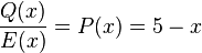
- In 1986, The Welch–Berlekamp algorithm was developed to solve the decoding equation of Reed–Solomon codes, using a fast method to solve a certain polynomial equation. The Berlekamp – Welch algorithm has a running time complexity of
 . We will in the following sections look at the Gemmel and Sudan’s exposition of the Berlekamp Welch Algorithm.[5]
Error locator polynomial of Reed–Solomon codes
In the problem of decoding Reed–Solomon codes, the inputs are pair wise distinct evaluation points  ’s (i = 1, . . ., n) where
  with dimension
  and distance
  and a codeword
  =
=  . Our goal is to describe an algorithm that can correct
  many errors in polynomial time. To do so we have to find a polynomial
  over
over  such that has degree less than
  and (the number of
  ’s such that
  . We can assume that there exists a polynomial
  such that
  ≤
≤  or
or  .
.
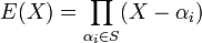
Note that the coefficients of are the encoded information. To solve this, we use an indicator for those ’s where an error may have occurred. Thus we define  , which is an error locator polynomial over such that
  if
if  and the degree of
  can be given by:
  .
.
-
 where
where 
We can also claim that for every  ,
,  . This fact holds true because in the event of , both sides of the above equation become
  because .
However since both and are unknown, the main task of the decoding algorithm would be to find . To do this we use a seemingly useless yet very powerful method and define another polynomial  as =
as =  . This is because the
  equations with
  we need to solve are quadratic in nature. Thus by defining a product of two variables that gives rise to a quadratic term as one unknown variable, we increase the number of unknowns but make the equations linear in nature. This method is called linearization[6] and is a very powerful tool.
Thus is a polynomial over having the properties:

This helps because if we now manage to find and , we can easily find using 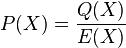 .
The main purpose of the Berlekamp Welch algorithm is to find out using degree bounded polynomials and and the properties of and
.
The main purpose of the Berlekamp Welch algorithm is to find out using degree bounded polynomials and and the properties of and  .
.
Computing is as hard as finding the end solution, polynomial . Once is computed, using erasure decoding for Reed–Solomon codes, we can easily recover . However in a few cases, even the polynomial is as hard to find as . As an example, given and (such that  for
for  ), by checking positions where
  , we can find the error locations. Thus the algorithm works on the principle that while each of the polynomials and are hard to find individually; computing them together is much easier.
The Berlekamp–Welch decoder and algorithm
The Welch–Berlekamp decoder for Reed–Solomon codes consists of the Welch– Berlekamp algorithm augmented by some additional steps that prepare the received word for the algorithm and interpret the result of the algorithm.
The inputs given to the Berlekamp Welch decoder are the integers denoting Block Length , the number of errors  such that < , and the received word
  satisfying the condition that there exists at most one with
  with
with 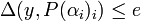 .
.
The output of the decoder is either the polynomial , or in some cases, a failure. This decoder functions in two steps as follows:
- This step is called the interpolation step in which the decoder computes a non zero polynomial of degree e (This implies that the coefficient of
 must be 1 [7]) and another polynomial with
 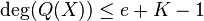 . These polynomials are created such that the condition
  for all . In the case that polynomials satisfying the above condition cannot be computed, the output of the decoder would be a failure.
 - If divides , then a ’
 is defined which equals
  . If
. If  ’
’ , then the decoder outputs ’. If the above condition is not satisfied, i.e. if does not divide then a failure is returned by the decoder.
According to the algorithm, in the cases where it does not output a failure, it outputs a that is the correct and desired polynomial. To prove that, the algorithm always outputs the desired polynomial, we need to prove a few claims we have made while describing the algorithm. Let us go ahead and do so now.
Claim 1: There exist a pair of polynomials and that satisfy Step 1 of the BW algorithm such that 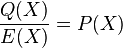 .
.
Let E(x) be the error-locating polynomial for such that  and let
  . Note that
  . We also stated that is a polynomial of degree exactly . Note that is a polynomial following the property that if and only if .We can now state that and satisfy the equation from the first step of the BW algorithm. If , then
  . However whenever
  , we can easily state that
  and therefore also state that
  just as we claimed.
This above claim however just reiterates and proves the fact that there exists a pair of polynomials and such that =  . It however does not necessarily guarantee the fact that the algorithm we discussed above would indeed output such a pair of polynomials. We therefore move on to look at another claim that helps establish this fact using the above claim and thereby proving the correctness of the algorithm.
Claim 2: For any two distinct solutions  that satisfy the first step of the Berlekamp Welch algorithm given above, they will also satisfy the equation
The total degrees of the polynomials  and
and  . We define another polynomial
  ....................................(i)
Note that  such that
  . From step 1 of the Berlekamp Welch algorithm we also know that
  and
and  ) ........…..........(ii)
Now, substituting the values of from equation (ii) into equation (i), we get:
 for .
for .
Thus, the above polynomial has roots and which implies that  < because of the upper bound on .
Since < , we can come to the conclusion that the polynomials
< because of the upper bound on .
Since < , we can come to the conclusion that the polynomials 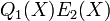 and
and  agree on more points than their degree, and hence they are identical. Note that since
  and
and  , it can be implied that as per our initial claim.
Thus based on the above claims, we can safely state that the output of the Berlekamp Welch algorithm, when outputting the polynomial is correct.
We can now claim that the algorithm can be implemented such that it has a running time of  . This can be proved as follows:
In Step 1 of the algorithm, the polynomials and have and
. This can be proved as follows:
In Step 1 of the algorithm, the polynomials and have and  unknown values respectively and the constraints for all acts as a linear equation with these unknowns. We therefore get a system of linear equations in
  <
<  unknowns. Using our first claim, this system of equations has a solution since the degree of polynomial is . This can be solved in time, by say Gaussian elimination. Finally, we can note that Step 2 of the algorithm can also be implemented in time by "long division" method.
Hence we can state that the Berlekamp Welch algorithm can be used to uniquely decode any
unknowns. Using our first claim, this system of equations has a solution since the degree of polynomial is . This can be solved in time, by say Gaussian elimination. Finally, we can note that Step 2 of the algorithm can also be implemented in time by "long division" method.
Hence we can state that the Berlekamp Welch algorithm can be used to uniquely decode any ![[n,k]_q](../I/m/0e2e8aa83a5c98cfb23abcec8cb69824.png) Reed–Solomon code in time for a maximum of
Reed–Solomon code in time for a maximum of  errors.
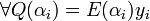
Example
_with_an_Error_Locator_Polynomial.png)
Consider a simple example where a redundant set of points are used to represent the line  , and one of the points is incorrect. The points that the algorithm gets as an input are
  , where
  is the defective point. The algorithm must solve the following system of equations:
Given a solution  and to this system of equations, it is evident that at any of the points
  one of the following must be true: either
  , or
, or 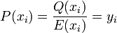 . Since is defined as only having a degree of one, the former can only be true in one point. Therefore,
  must equal
  at the three other points.
Letting  and
and  and bringing
  to the left, we can rewrite the system thus:
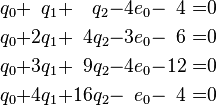
This system can be solved through Gaussian elimination, and gives the values:

Thus,  . Dividing the two gives:
 fits three of the four points given, so it is the most likely to be the original polynomial.
See also
References
- ↑ Berlekamp, Elwyn R. (1967), Nonbinary BCH decoding, International Symposium on Information Theory, San Remo, Italy
- ↑ Berlekamp, Elwyn R. (1984) [1968], Algebraic Coding Theory (Revised ed.), Laguna Hills, CA: Aegean Park Press, ISBN 0-89412-063-8. Previous publisher McGraw–Hill, New York, NY.
- ↑ Massey, J. L. (1969), "Shift-register synthesis and BCH decoding", IEEE Trans. Information Theory, IT-15 (1): 122–127
- ↑ Ben Atti, Nadia; Diaz-Toca, Gema M.; Lombardi, Henri, The Berlekamp–Massey Algorithm revisited, CiteSeerX: 10
.1 .1 .96 .2743 - ↑ Highly resilient correctors for polynomials – Peter Gemmel and Madhu Sudan's Exposition.
- ↑ A provable example of the linearization method – Dick Lipton
- ↑ Atri, Rudra. "Error Correcting Codes: Combinatorics, Algorithms and Applications". CSE_BUFFALO. Retrieved 2014-12-12.
External links
- MIT Lecture Notes on Essential Coding Theory – Dr. Madhu Sudan
- University at Buffalo Lecture Notes on Coding Theory – Dr. Atri Rudra
- Algebraic Codes on Lines, Planes and Curves, An Engineering Approach – Richard E. Blahut
- Welch Berlekamp Decoding of Reed–Solomon Codes – L. R. Welch
- US 4,633,470, Welch, Lloyd R. & Elwyn R. Berlekamp, "Error Correction for Algebraic Block Codes", published September 27, 1983, issued December 30, 1986 – The patent by Lloyd R. Welch and Elewyn R. Berlekamp