Autoregressive fractionally integrated moving average
In statistics, autoregressive fractionally integrated moving average models are time series models that generalize ARIMA (autoregressive integrated moving average) models by allowing non-integer values of the differencing parameter. These models are useful in modeling time series with long memory—that is, in which deviations from the long-run mean decay more slowly than an exponential decay. The acronyms "ARFIMA" or "FARIMA" are often used, although it is also conventional to simply extend the "ARIMA(p,d,q)" notation for models, by simply allowing the order of differencing, d, to take fractional values.
Basics
In an ARIMA model, the integrated part of the model includes the differencing operator (1 − B) (where B is the backshift operator) raised to an integer power. For example
where
so that
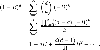
In a fractional model, the power is allowed to be fractional, with the meaning of the term identified using the following formal binomial series expansion
ARFIMA(0,d,0)
The simplest autoregressive fractionally integrated model, ARFIMA(0,d,0), is, in standard notation,
where this has the interpretation
ARFIMA(0,d,0) is similar to fractional Gaussian noise (fGn): with d = H−½, their covariances have the same power-law decay. The advantage of fGn over ARFIMA(0,d,0) is that many asymptotic relations hold for finite samples.[1] The advantage of ARFIMA(0,d,0) over fGn is that it has an especially simple spectral density—
- f(λ) = (1/2π) (2sin(λ/2))−2d
—and it is a particular case of ARFIMA(p,d,q), which is a versatile family of models.[1]
General form: ARFIMA(p,d,q)
An ARFIMA model shares the same form of representation as the ARIMA(p,d,q) process, specifically:
In contrast to the ordinary ARIMA process, the "difference parameter", d, is allowed to take non-integer values.
See also
- Fractional calculus — fractional differentiation
- Differintegral — fractional integration and differentiation
- Fractional Brownian motion — a continuous-time stochastic process with a similar basis
- Long-range dependency
Notes
- ↑ 1.0 1.1 Taqqu, M. S.; Teverovsky, V.; Willinger, W. (1995). "Estimators for Long-Range Dependence: An Empirical Study". Fractals 3 (4): 785–798. doi:10.1142/S0218348X95000692.
References
- Granger, C. W. J.; Joyeux, R. (1980). "An introduction to long-memory time series models and fractional differencing". Journal of Time Series Analysis 1: 15–30. doi:10.1111/j.1467-9892.1980.tb00297.x.
- Hosking, J. R. M. (1981). "Fractional differencing". Biometrika 68 (1): 165–176. doi:10.1093/biomet/68.1.165.
- Robinson, P. M. (2003). Time Series With Long Memory. Oxford University Press. ISBN 0-19-925729-9.


