Artin transfer (group theory)
In the mathematical field of group theory, an Artin transfer is a certain homomorphism from a group to the commutator quotient group of a subgroup of finite index. Originally, such mappings arose as group theoretic counterparts of class extension homomorphisms of abelian extensions of algebraic number fields by applying Artin's reciprocity maps to ideal class groups and analyzing the resulting homomorphisms between quotients of Galois groups. However, independently of number theoretic applications, the kernels and targets of Artin transfers have recently turned out to be compatible with parent-descendant relations between finite p-groups, which can be visualized in descendant trees. Therefore, Artin transfers provide a valuable tool for the classification of finite p-groups and for searching particular groups in descendant trees by looking for patterns defined by the kernels and targets of Artin transfers. These methods of pattern recognition are useful in purely group theoretic context, as well as for applications in algebraic number theory concerning higher p-class groups and Hilbert p-class field towers.
Transversals of a subgroup
Let  be a group and
  be a subgroup of finite index
  .
.
Definitions. [1]
- A left transversal of
 in is an ordered system
  of representatives for the left cosets of in such that
  is a disjoint union.
 - Similarly, a right transversal of in is an ordered system
 of representatives for the right cosets of in such that
  is a disjoint union.
- A left transversal of
Remarks. [2]
- For any transversal of in , there exists a unique subscript
 such that
  , resp.
  . Of course, this element may be, but need not be, replaced by the neutral element
  .
. - If is non-abelian and is not a normal subgroup of , then we can only say that the inverse elements
 of a left transversal form a right transversal of in , since implies
  .
. - However, if
 is a normal subgroup of , then any left transversal is also a right transversal of in , since
  for each
  .
.
- For any transversal of
Permutation representation
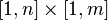
Suppose is a left transversal of a subgroup of finite index in a group .
A fixed element gives rise to a unique permutation  of the left cosets of in such that
 , resp.
 , resp.
 , for each
  .
.
Similarly, if is a right transversal of in , then
a fixed element gives rise to a unique permutation  of the right cosets of in such that
 , resp.
 , resp.
 , for each .
Definition. [1]
The mapping  , resp.
  , is called the permutation representation of in
  with respect to , resp. .
The mapping
 , resp.
 , is called the monomial representation of in
  with respect to , resp. .
Remark.
For the special right transversal associated to the left transversal we have
 but on the other hand
 , for each .
This relation simultaneously shows that, for any , the associated permutation representations are connected by
, for each .
This relation simultaneously shows that, for any , the associated permutation representations are connected by  ,
and the associated monomial representations are connected additionally by
,
and the associated monomial representations are connected additionally by  , for each .
Artin transfer
Let be a group and be a subgroup of finite index .
Assume that , resp. , is a left, resp. right, transversal of in .
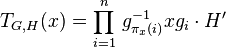
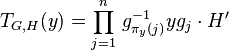
Then the Artin transfer  from to the abelianization of with respect to , resp. , is defined by
  or briefly
  , resp.
  or briefly
  , for .
Independence of the transversal
Assume that  is another left transversal of in
such that
is another left transversal of in
such that  .
Then there exists a unique permutation
.
Then there exists a unique permutation  such that
  , for all .
Consequently,
, for all .
Consequently,  , resp.
  with
with  ,
for all .
For a fixed element , there exists a unique permutation
,
for all .
For a fixed element , there exists a unique permutation  such that we have
 ,
for all .
Therefore, the permutation representation of with respect to is given by
,
for all .
Therefore, the permutation representation of with respect to is given by
 , resp.
 , for .
Furthermore, for the connection between the elements
, for .
Furthermore, for the connection between the elements
 and , we obtain

 ,
for all .
Finally, due to the commutativity of the quotient group
,
for all .
Finally, due to the commutativity of the quotient group  and the fact that
  are permutations, the Artin transfer turns out to be independent of the left transversal:
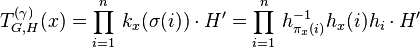
 , as defined above.
It is clear that a similar proof shows that the Artin transfer is independent of the choice between two different right transversals.
It remains to show that the Artin transfer with respect to a right transversal coincides with the Artin transfer with respect to a left transversal. For this purpose, we select the special right transversal associated to the left transversal . Using the commutativity of and the remark in the previous section, we consider the expression

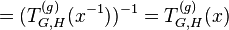 . The last step is justified by the fact that the Artin transfer is a homomorphism. This will be shown in the following section.
Homomorphisms
Let  be two elements with transfer images
 and
and
 .
Since is abelian and
.
Since is abelian and  is a permutation,
we can change the order of the factors in the following product:
is a permutation,
we can change the order of the factors in the following product:

 .
This relation simultaneously shows that the Artin transfer
.
This relation simultaneously shows that the Artin transfer  and the permutation representation are homomorphisms,
since
and the permutation representation are homomorphisms,
since  .
.
It is illuminating to restate the homomorphism property of the Artin transfer in terms of the monomial representation. The images of the factors  are given by
and
are given by
and
 .
The image of the product
.
The image of the product  turned out to be
 ,
which is a very peculiar law of composition discussed in more detail in the following section.
,
which is a very peculiar law of composition discussed in more detail in the following section.
The law reminds of the crossed homomorphisms  in the first cohomology group
  of a -module
  , which have the property
 .
.
Wreath product of H and S(n)
The peculiar structures which arose in the previous section can also be interpreted by endowing the cartesian product with a special law of composition known as the wreath product  of the groups and with respect to the set
  .
For , it is given by
.
For , it is given by


 ,
which causes the monomial representation
,
which causes the monomial representation
 also to be a homomorphism.
In fact, it is an injective homomorphism, also called a monomorphism or embedding,
in contrast to the permutation representation.
also to be a homomorphism.
In fact, it is an injective homomorphism, also called a monomorphism or embedding,
in contrast to the permutation representation.
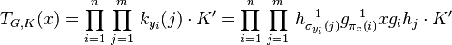
Composition
Let be a group with nested subgroups  such that the index
  is finite. Then the Artin transfer
  is the compositum of the induced transfer
  and the Artin transfer , that is,
  . This can be seen in the following manner.
If is a left transversal of in and 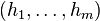 is a left transversal of
  in , that is
 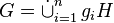 and
and 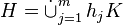 , then
  is a disjoint left coset decomposition of with respect to . Given two elements and
  , there exist unique permutations , and
  , such that , for each , and
 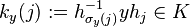 , for each
  . Then , and
 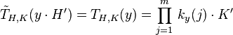 . For each pair of subscripts and , we have
  , resp.
 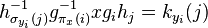 , where
  . Therefore, the image of
  under the Artin transfer is given by
 .
.
Finally, we want to emphasize the structural peculiarity of the corresponding monomial representation
 ,
,
 ,
defining
,
defining
 for a permutation
 ,
and using the symbolic notation
,
and using the symbolic notation  for all pairs of subscripts , .
The preceding proof has shown that
 .
Therefore, the action of the permutation
.
Therefore, the action of the permutation  on the set
 is given by
 .
The action on the second component depends on the first component
(via the permutation
.
The action on the second component depends on the first component
(via the permutation  to be selected)
whereas the action on the first component is independent of the second component.
Therefore, the permutation can be identified with the multiplet
to be selected)
whereas the action on the first component is independent of the second component.
Therefore, the permutation can be identified with the multiplet

which will be written in twisted form in the next section.
Wreath product of S(m) and S(n)
The permutations , which arose as second components of the monomial representation
,
,
in the previous section, are of a very special kind.
They belong to the stabilizer of the natural equipartition of the set
into the  rows of the corresponding matrix (rectangular array).
Using the peculiarities of the composition of Artin transfers in the previous section,
we show that this stabilizer is isomorphic to the wreath product
rows of the corresponding matrix (rectangular array).
Using the peculiarities of the composition of Artin transfers in the previous section,
we show that this stabilizer is isomorphic to the wreath product
 of the groups
  and with respect to the set , whose underlying set
  is endowed with the following law of composition


 for all
  .
.
This law reminds of the chain rule
 for the Fréchet derivative in
  of the compositum of differentiable functions
 and
and  between normed spaces.
The above considerations establish a third representation, the stabilizer representation,
 of the group in the wreath product ,
similar to the permutation representation and the monomial representation.
As opposed to the latter, the stabilizer representation cannot be injective, in general.
For instance, if is infinite.
of the group in the wreath product ,
similar to the permutation representation and the monomial representation.
As opposed to the latter, the stabilizer representation cannot be injective, in general.
For instance, if is infinite.
Cycle decomposition
Let be a left transversal of a subgroup of finite index in a group .
Suppose the element gives rise to the permutation of the left cosets of in such that
, resp.  , for each .
If  has the decomposition
  into pairwise disjoint cycles
  of lengths
  , which is unique up to the ordering of the cycles, more explicitly, if
  , for
, for  , and
, and  , then the image of under the Artin transfer is given by
  .
.
The reason for this fact is that we obtain another left transversal of in by putting  for
for  and , since
  . Let us fix a value of . For
  , we have
  , resp.
  . However, for
  , we obtain
  , resp.
  . Consequently,
  .
The cycle decomposition corresponds to a double coset decomposition
.
The cycle decomposition corresponds to a double coset decomposition  of the group modulo the cyclic group
  and the subgroup . It was actually this cycle decomposition form of the transfer homomorphism which was given by E. Artin in his original 1929 paper.[3]
Normal subgroup
Let be a normal subgroup of finite index in a group . Then we have , for all , and there exists the quotient group  of order . For an element , we let
  denote the order of the coset
  in . Then,
  is a cyclic subgroup of order
  of , and a (left) transversal
  of the subgroup
  in , where
  and
and  , can be extended to a (left) transversal
 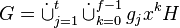 of in . Hence, the formula for the image of under the Artin transfer in the previous section takes the particular shape
 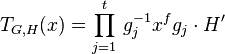 with exponent independent of
  .
.
In particular, the inner transfer of an element  of order
  is given as a symbolic power
 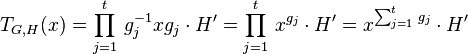 with the trace element
 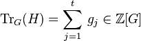 of in as symbolic exponent.
The other extreme is the outer transfer of an element
of in as symbolic exponent.
The other extreme is the outer transfer of an element  which generates modulo , that is
  and
and  . It is simply an th power
  .
.
Explicit implementations of Artin transfers in the simplest situations are presented in the following section.
Computational implementation
Abelianization of type (p,p)
Let be a p-group with abelianization  of elementary abelian type
  . Then has
  maximal subgroups
 of index
  . For each
  , let
, let 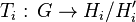 be the Artin transfer homomorphism from to the abelianization of
  . According to Burnside's basis theorem, the group has generator rank
  and can therefore be generated as
  by two elements such that
  . For each of the normal subgroups
  , a generator
  with respect to
  , and a generator
  of a transversal must be given such that
 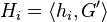 and
and  . A convenient selection is given by
  ,
,  , and
, and  ,
,  , for all
 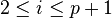 . Then, for each , it is sufficient to define the inner transfer by
  , which can also be expressed as a product of two pth powers
  , and the outer transfer as a complete pth power by
 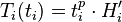 . The reason is that
  and
and  . It should be pointed out that the complete specification of the Artin transfers also requires explicit knowledge of the derived subgroups
  . Since is a normal subgroup of index
  in , a certain general reduction is possible by
  ,
[4]
but a presentation of must be known for determining generators of
,
[4]
but a presentation of must be known for determining generators of  , whence
  .
.
Abelianization of type (p2,p)
Let be a p-group with abelianization of non-elementary abelian type  . Then has maximal subgroups of index and subgroups
  of index
 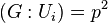 . For each , let
 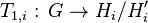 , resp.
 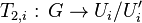 , be the Artin transfer homomorphism from to the abelianization of , resp.
  . Burnside's basis theorem asserts that the group has generator rank and can therefore be generated as by two elements such that
  . We begin by considering the first layer of subgroups. For each of the normal subgroups
  , we select a generator
  such that . These are the cases where the factor group
  is cyclic of order
  . However, for the distinguished maximal subgroup
  , for which the factor group
  is bicyclic of type , we need two generators
  and
and  such that
 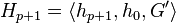 . Further, a generator of a transversal must be given such that , for each . It is convenient to define , for
  , and
, and  . Then, for each , we have the inner transfer
  , which equals
  , and the outer transfer
  , since and . Now we continue by considering the second layer of subgroups. For each of the normal subgroups
  , we select a generator
  ,
,  for
for  , and
, and  , such that
  . Among these subgroups, the Frattini subgroup
  is particularly distinguished. A uniform way of defining generators
  of a transversal such that
  , is to set
  , for , and
  . Since
  , but on the other hand
  and
and  , for , with the single exception that
  , we obtain the following expressions for the inner transfer
  , and for the outer transfer
  , exceptionally
  , and
, and  , for . Again, it should be emphasized that the structure of the derived subgroups and
  must be known to specify the action of the Artin transfers completely.
Transfer kernels and targets
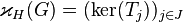
Let be a group with finite abelianization . Suppose that  denotes the family of all subgroups which contain the commutator subgroup and are therefore necessarily normal, enumerated by means of the finite index set
  . For each
  , let
, let  be the Artin transfer from to the abelianization
  .
.
Definition. [5]
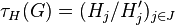
The family of normal subgroups  is called the transfer kernel type (TKT) of with respect to , and the family of abelianizations (resp. their abelian type invariants)
  is called the transfer target type (TTT) of with respect to .
Both families are also called multiplets whereas a single component will be referred to as a singulet.
is called the transfer target type (TTT) of with respect to .
Both families are also called multiplets whereas a single component will be referred to as a singulet.
Important examples for these concepts are provided in the following two sections.
Abelianization of type (p,p)
Let be a p-group with abelianization of elementary abelian type . Then has maximal subgroups of index . For each , let be the Artin transfer homomorphism from to the abelianization of .
Definition.
The family of normal subgroups  is called the transfer kernel type (TKT) of with respect to
  .
.
Remarks.
- For brevity, the TKT is identified with the multiplet
 , whose integer components are given by
  Here, we take into consideration that each transfer kernel
  must contain the commutator subgroup of , since the transfer target is abelian. However, the minimal case
  cannot occur.
 - A renumeration of the maximal subgroups
 and of the transfers
  by means of a permutation
  gives rise to a new TKT
  with respect to
  , identified with
 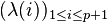 , where
 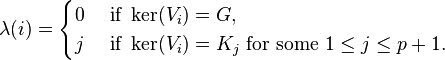 It is adequate to view the TKTs
 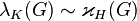 as equivalent. Since we have
  , the relation between
  and
and  is given by
  . Therefore, is another representative of the orbit
  of under the operation
  of the symmetric group
  on the set of all mappings from
  to
to  , where the extension
  of the permutation is defined by
  , and formally
  ,
,  .
.
- For brevity, the TKT is identified with the multiplet
Definition.
The orbit  of any representative is an invariant of the p-group and is called its transfer kernel type, briefly TKT.
Remark.
Let  denote the counter of total transfer kernels
  , which is an invariant of the group .
In 1980, S. M. Chang and R. Foote
[6]
proved that, for any odd prime and for any integer
, which is an invariant of the group .
In 1980, S. M. Chang and R. Foote
[6]
proved that, for any odd prime and for any integer  ,
there exist metabelian p-groups having abelianization of type such that
,
there exist metabelian p-groups having abelianization of type such that  .
However, for
.
However, for  , there do not exist non-abelian
  -groups with
  , which must be metabelian of maximal class, such that
  . Only the elementary abelian -group
  has
has  . See Figure 5.
In the following concrete examples for the counters  , and also in the remainder of this article, we use identifiers of finite p-groups in the SmallGroups Library by H. U. Besche, B. Eick and E. A. O'Brien
.[7]
[8]
, and also in the remainder of this article, we use identifiers of finite p-groups in the SmallGroups Library by H. U. Besche, B. Eick and E. A. O'Brien
.[7]
[8]
For  , we have
-
 for the extra special group
  of exponent
  with TKT
  (Figure 6),
 -
 for the two groups
  with TKTs
  (Figures 8 and 9),
 -
 for the group
  with TKT
  (Figure 4 in the article on descendant trees),
 - for the group
 with TKT
  (Figure 6),
 -
 for the extra special group
  of exponent
  with TKT
  (Figure 6).
-
Abelianization of type (p2,p)
Let be a p-group with abelianization of non-elementary abelian type . Then possesses maximal subgroups of index , and subgroups of index .
Assumption.
Suppose that  is the distinguished maximal subgroup which is the product of all subgroups of index , and
  is the distinguished subgroup of index which is the intersection of all maximal subgroups, that is the Frattini subgroup
  of .
of .
First layer
For each , let be the Artin transfer homomorphism from to the abelianization of .
Definition.
The family  is called the first layer transfer kernel type of with respect to and
  , and is identified with
 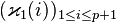 , where
Remark.
Here, we observe that each first layer transfer kernel is of exponent with respect to and consequently cannot coincide with  for any
  , since
  is cyclic of order , whereas is bicyclic of type .
Second layer
For each , let be the Artin transfer homomorphism from to the abelianization of .
Definition.
The family  is called the second layer transfer kernel type of with respect to and , and is identified with
 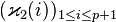 , where
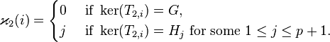
Transfer kernel type
Combining the information on the two layers, we obtain the (complete) transfer kernel type  of the p-group with respect to and .
Remark.
The distinguished subgroups and  are unique invariants of and should not be renumerated. However, independent renumerations of the remaining maximal subgroups
  and the transfers
  by means of a permutation
  , and of the remaining subgroups
  of index and the transfers
  by means of a permutation
  , give rise to new TKTs
  with respect to and
  , identified with
  , where
 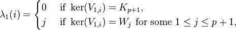 and
and  with respect to and , identified with
 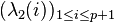 , where
 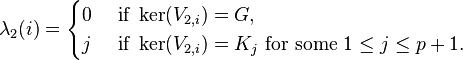 It is adequate to view the TKTs
  and
and  as equivalent. Since we have
  , resp.
  , the relations between
  and
and  , resp.
  and
and  , are given by
  , resp.
  . Therefore,
  is another representative of the orbit
  of
of  under the operation
  of the product of two symmetric groups
  on the set of all pairs of mappings from to , where the extensions
  and of a permutation
  are defined by
  and , and formally
  ,
,  ,
,  , and
, and  .
.
Definition.
The orbit  of any representative is an invariant of the p-group and is called its transfer kernel type, briefly TKT.
Connections between layers
The Artin transfer from to a subgroup of index () is the compositum  of the induced transfer
  from to and the Artin transfer
  from to , for any intermediate subgroup
 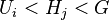 of index
  (
( ). There occur two situations:
- For the subgroups
 only the distinguished maximal subgroup is an intermediate subgroup.
 - For the Frattini subgroup all maximal subgroups are intermediate subgroups.
- For the subgroups
This causes restrictions for the transfer kernel type  of the second layer, since
  , and thus
-
 , for all ,
 - but even
 .
.
-
Furthermore, when with  and
and  , an element
  (
( ) which is of order with respect to , can belong to the transfer kernel
  only if its th power
  is contained in
  , for all intermediate subgroups , and thus:
-
 , for certain
  , enforces the first layer TKT singulet
  ,
, - but
 , for some , even specifies the complete first layer TKT multiplet
  , that is
  , for all .
-
Inheritance from quotients
The common feature of all parent-descendant relations between finite p-groups is that the parent  is a quotient
  of the descendant by a suitable normal subgroup
  . Thus, an equivalent definition can be given by selecting an epimorphism
  from onto a group
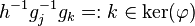
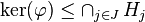
  whose kernel
  plays the role of the normal subgroup . In the following sections, this point of view will be taken, generally for arbitrary groups.
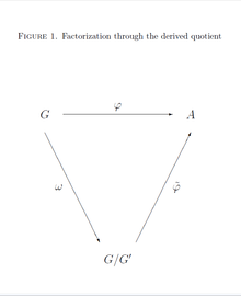
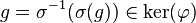
Passing through the abelianization
If  is a homomorphism from a group to an abelian group
  , then there exists a unique homomorphism
  such that
  , where
  denotes the canonical projection. The kernel of
  is given by
  . The situation is visualized in Figure 1.
The uniqueness of is a consequence of the condition , which implies that must be defined by  , for any . The relation
  , for , shows that is a homomorphism. For the commutator of , we have
  , since is abelian. Thus, the commutator subgroup of is contained in the kernel , and this finally shows that the definition of is independent of the coset representative,


 .
.
TTT singulets
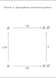
Let and be groups such that  is the image of under an epimorphism
  and
and  is the image of a subgroup
  .
.
The commutator subgroup of  is the image of the commutator subgroup of , that is
  .
If
.
If  , then
  , induces a unique epimorphism
  , and thus
  is epimorphic image of , that is a quotient of .
Moreover, if even
is epimorphic image of , that is a quotient of .
Moreover, if even  , then
 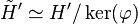 , the map is an isomorphism, and
 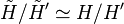 .
See Figure 2 for a visualization of this scenario.
.
See Figure 2 for a visualization of this scenario.
The statements can be seen in the following manner.
The image of the commutator subgroup is 
 .
If , then can be restricted to an epimorphism
.
If , then can be restricted to an epimorphism 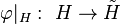 , whence
 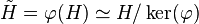 . According to the previous section, the composite epimorphism
 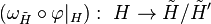 from onto the abelian group factors through by means of a uniquely determined epimorphism such that
 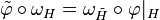 . Consequently, we have
 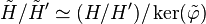 . Furthermore, the kernel of is given explicitly by
  .
Finally, if , then
.
Finally, if , then 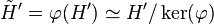 and is an isomorphism, since
  .
.
Definition. [9]
Due to the results in the present section, it makes sense to define a partial order on the set of abelian type invariants by putting
 , when , and
 , when .
TKT singulets
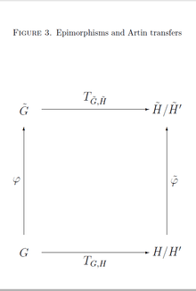
Suppose that and are groups, is the image of under an epimorphism , and is the image of a subgroup of finite index . Let be the Artin transfer from to and  be the Artin transfer from to .
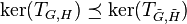
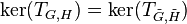
If , then the image 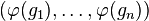 of a left transversal of in is a left transversal of in , and the inclusion
 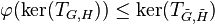 holds.
Moreover, if even , then the equation
holds.
Moreover, if even , then the equation  holds.
See Figure 3 for a visualization of this scenario.
holds.
See Figure 3 for a visualization of this scenario.
The truth of these statements can be justified in the following way.
Let be a left transversal of in . Then is a disjoint union but  is not necessarily disjoint. For
  , we have


 for some element
 . However, if the condition is satisfied, then we are able to conclude that
  , and thus
  .
.
Let be the epimorphism obtained in the manner indicated in the previous section.
For the image of under the Artin transfer, we have  . Since
  , the right hand side equals
  , provided that is a left transversal of in , which is correct, when . This shows that the diagram in Figure 3 is commutative, that is
 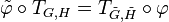 .
Consequently, we obtain the inclusion , if .
Finally, if , then the previous section has shown that is an isomorphism. Using the inverse isomorphism, we get
.
Consequently, we obtain the inclusion , if .
Finally, if , then the previous section has shown that is an isomorphism. Using the inverse isomorphism, we get 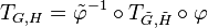 , which proves the equation .
Definition. [9]
In view of the results in the present section, we are able to define a partial order of transfer kernels by setting
 , when , and
 , when .
TTT and TKT multiplets
Suppose and are groups, is the image of under an epimorphism , and both groups have isomorphic finite abelianizations 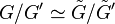 .
Let denote the family of all subgroups which contain the commutator subgroup (and thus are necessarily normal), enumerated by means of the finite index set , and let
.
Let denote the family of all subgroups which contain the commutator subgroup (and thus are necessarily normal), enumerated by means of the finite index set , and let  be the image of under , for each .
Assume that, for each , denotes the Artin transfer from to the abelianization , and
be the image of under , for each .
Assume that, for each , denotes the Artin transfer from to the abelianization , and  denotes the Artin transfer from to the abelianization
  .
Finally, let
.
Finally, let  be any non-empty subset of .
Then it is convenient to define
 , called the (partial) transfer kernel type (TKT) of with respect to
  , and
, and
 , called the (partial) transfer target type (TTT) of with respect to .
Due to the rules for singulets, established in the preceding two sections, these multiplets of TTTs and TKTs obey the following fundamental inheritance laws:
- If
 , then
 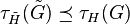 , in the sense that
  , for each
  , and
, and  , in the sense that
  , for each .
 - If
 , then
  , in the sense that
  , for each , and
  , in the sense that
  , for each .
- If
Inherited automorphisms
A further inheritance property does not immediately concern Artin transfers but will prove to be useful in applications to descendant trees.
Let and be groups such that 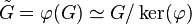 is the image of under an epimorphism . Suppose that
  is an automorphism of .
If 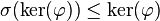 , then there exists a unique epimorphism
  such that
 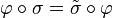 . If
. If 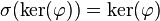 , then
  is also an automorphism.
The justification for these facts is based on the isomorphic representation , which permits to identify  for all
  and proves the uniqueness of
  . If , then the consistency follows from
 . And if , then injectivity of is a consequence of
 , since
  .
.
Now, let us denote the canonical projection from to its abelianization by  .
There exists a unique induced automorphism
.
There exists a unique induced automorphism  such that
  , that is,
  , for all .
The reason for the injectivity of
, for all .
The reason for the injectivity of  is that

 , since is a characteristic subgroup of .
Definition.
is called a σ-group, if there exists an automorphism such that the induced automorphism acts like the inversion on , that is,  , resp.
  , for all .
The supplementary inheritance property asserts that, if is a  -group and , then is also a -group, the required automorphism being .
This can be seen by applying the epimorphism to the equation , for , which yields  , for all
  .
.
Stabilization criteria
In this section, the results concerning the inheritance of TTTs and TKTs from quotients in the previous section are applied to the simplest case, which is characterized by the following
Assumption.
The parent of a group is the quotient  of by the last non-trivial term
  of the lower central series of , where
  denotes the nilpotency class of . The corresponding epimorphism
  from onto
  is the canonical projection, whose kernel is given by
  .
.
Under this assumption, the kernels and targets of Artin transfers turn out to be compatible with parent-descendant relations between finite p-groups.
Compatibility criterion.
Let be a prime number. Suppose that is a non-abelian finite p-group of nilpotency class  . Then the TTT and the TKT of and of its parent are comparable in the sense that
  and
and  .
.
The simple reason for this fact is that, for any subgroup  , we have
  , since
  .
.
For the remaining part of this section,
the investigated groups are supposed to be finite metabelian p-groups with elementary abelianization of rank , that is of type .
Partial stabilization for maximal class.
A metabelian p-group of coclass  and of nilpotency class
  shares the last components of the TTT
  and of the TKT
  with its parent .
More explicitly, for odd primes
with its parent .
More explicitly, for odd primes  , we have
  and
and  for .
[10]
for .
[10]
This criterion is due to the fact that  implies
  ,
[11]
for the last maximal subgroups
,
[11]
for the last maximal subgroups  of .
of .
The condition is indeed necessary for the partial stabilization criterion. For odd primes , the extra special -group  of order
  and exponent has nilpotency class
  only, and the last components of its TKT
  are strictly smaller than the corresponding components of the TKT
  of its parent which is the elementary abelian -group of type .
[10]
For , both extra special -groups of coclass and class , the ordinary quaternion group with TKT
of its parent which is the elementary abelian -group of type .
[10]
For , both extra special -groups of coclass and class , the ordinary quaternion group with TKT  and the dihedral group
  with TKT
  , have strictly smaller last two components of their TKTs than their common parent
  with TKT
  .
.
Total stabilization for maximal class and positive defect.
A metabelian p-group of coclass and of nilpotency class  , that is, with index of nilpotency
  , shares all components of the TTT and of the TKT with its parent , provided it has positive defect of commutativity
  .
[5]
Note that
.
[5]
Note that  implies , and we have for all .
[10]
implies , and we have for all .
[10]
This statement can be seen by observing that the conditions and imply  ,
[11]
for all the maximal subgroups of .
,
[11]
for all the maximal subgroups of .
The condition is indeed necessary for total stabilization. To see this it suffices to consider the first component of the TKT only. For each nilpotency class  , there exist (at least) two groups
  with TKT
  and
and  with TKT
  , both with defect
  , where the first component of their TKT is strictly smaller than the first component of the TKT of their common parent
  .
.
Partial stabilization for non-maximal class.
Let be fixed.
A metabelian 3-group with abelianization  , coclass
  and nilpotency class
  shares the last two (among the four) components of the TTT and of the TKT with its parent .
This criterion is justified by the following consideration. If , then  [11]
for the last two maximal subgroups
[11]
for the last two maximal subgroups  of .
of .
The condition is indeed unavoidable for partial stabilization, since there exist several -groups of class  , for instance those with SmallGroups identifiers
  , such that the last two components of their TKTs
  are strictly smaller than the last two components of the TKT of their common parent
  .
.
Total stabilization for non-maximal class and cyclic centre.
Again, let be fixed.
A metabelian 3-group with abelianization , coclass , nilpotency class and cyclic centre  shares all four components of the TTT and of the TKT with its parent .
The reason is that, due to the cyclic centre, we have  [11]
for all four maximal subgroups
[11]
for all four maximal subgroups  of .
of .
The condition of a cyclic centre is indeed necessary for total stabilization, since for a group with bicyclic centre there occur two possibilities.
Either  is also bicyclic, whence
  is never contained in
  ,
or
,
or  is cyclic but is never contained in
  .
.
Summarizing, we can say that the last four criteria underpin the fact that Artin transfers provide a marvellous tool for classifying finite p-groups.
In the following sections, it will be shown how these ideas can be applied for endowing descendant trees with additional structure, and for searching particular groups in descendant trees by looking for patterns defined by the kernels and targets of Artin transfers. These strategies of pattern recognition are useful in pure group theory and in algebraic number theory.
Structured descendant trees (SDTs)
This section uses the terminology of descendant trees in the theory of finite p-groups.
In Figure 4, a descendant tree with modest complexity is selected exemplarily to demonstrate how Artin transfers provide additional structure for each vertex of the tree.
More precisely, the underlying prime is , and the chosen descendant tree is actually a coclass tree having a unique infinite mainline, branches of depth , and strict periodicity of length setting in with branch  .
The initial pre-period consists of branches
.
The initial pre-period consists of branches  and
and  with exceptional structure.
Branches and
with exceptional structure.
Branches and  form the primitive period such that
  , for odd
  , and
, and  , for even
  .
The root of the tree is the metabelian -group with identifier
.
The root of the tree is the metabelian -group with identifier  , that is, a group of order
  and with counting number
  . It should be emphasized that this root is not coclass settled, whence its entire descendant tree
  is of considerably higher complexity than the coclass- subtree
  , whose first six branches are drawn in the diagram of Figure 4.
The additional structure can be viewed as a sort of coordinate system in which the tree is embedded. The horizontal abscissa is labelled with the transfer kernel type (TKT) , and the vertical ordinate is labelled with a single component
, whose first six branches are drawn in the diagram of Figure 4.
The additional structure can be viewed as a sort of coordinate system in which the tree is embedded. The horizontal abscissa is labelled with the transfer kernel type (TKT) , and the vertical ordinate is labelled with a single component  of the transfer target type (TTT). The vertices of the tree are drawn in such a manner that members of periodic infinite sequences form a vertical column sharing a common TKT. On the other hand, metabelian groups of a fixed order, represented by vertices of depth at most , form a horizontal row sharing a common first component of the TTT. (To discourage any incorrect interpretations, we explicitly point out that the first component of the TTT of non-metabelian groups or metabelian groups, represented by vertices of depth , is usually smaller than expected, due to stabilization phenomena!) The TTT of all groups in this tree represented by a big full disk, which indicates a bicyclic centre of type
  , is given by
  with varying first component
  , the nearly homocyclic abelian -group of order
  , and fixed further components
  and
and  , where the abelian type invariants are either written as orders of cyclic components or as their -logarithms with exponents indicating iteration. (The latter notation is employed in Figure 4.) Since the coclass of all groups in this tree is , the connection between the order
  and the nilpotency class is given by
  .
.
Pattern recognition
For searching a particular group in a descendant tree by looking for patterns defined by the kernels and targets of Artin transfers, it is frequently adequate to reduce the number of vertices in the branches of a dense tree with high complexity by sifting groups with desired special properties, for example
- filtering the -groups,
- eliminating a set of certain transfer kernel types,
- cancelling all non-metabelian groups (indicated by small contour squares in Fig. 4),
- removing metabelian groups with cyclic centre (denoted by small full disks in Fig. 4),
- cutting off vertices whose distance from the mainline (depth) exceeds some lower bound,
- combining several different sifting criteria.
- filtering the
The result of such a sieving procedure is called a pruned descendant tree with respect to the desired set of properties.
However, in any case, it should be avoided that the main line of a coclass tree is eliminated, since the result would be a disconnected infinite set of finite graphs instead of a tree.
For example, it is neither recommended to eliminate all -groups in Figure 4 nor to eliminate all groups with TKT  .
In Figure 4, the big double contour rectangle surrounds the pruned coclass tree
.
In Figure 4, the big double contour rectangle surrounds the pruned coclass tree  , where the numerous vertices with TKT
  are completely eliminated. This would, for instance, be useful for searching a -group with TKT
  and first component
  of the TTT. In this case, the search result would even be a unique group. We expand this idea further in the following detailed discussion of an important example.
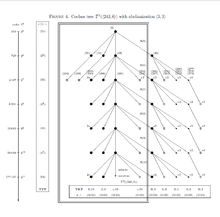
Historical example
The oldest example of searching for a finite p-group by the strategy of pattern recognition via Artin transfers goes back to 1934, when A. Scholz and O. Taussky
[12]
tried to determine the Galois group  of the Hilbert -class field tower, that is the maximal unramified pro- extension
  , of the complex quadratic number field
  .
They actually succeeded in finding the maximal metabelian quotient
.
They actually succeeded in finding the maximal metabelian quotient  of , that is the Galois group of the second Hilbert -class field
  of .
However, it needed
of .
However, it needed  years until M. R. Bush and D. C. Mayer, in 2012, provided the first rigorous proof
[9]
that the (potentially infinite) -tower group
years until M. R. Bush and D. C. Mayer, in 2012, provided the first rigorous proof
[9]
that the (potentially infinite) -tower group  coincides with the finite -group
  of derived length
  , and thus the -tower of has exactly three stages, stopping at the third Hilbert -class field
  of .
of .
| c | order of Pc |
SmallGroups identifier of Pc |
TKT of Pc |
TTT  of Pc |
ν | μ | descendant numbers of Pc |
|---|---|---|---|---|---|---|---|
| | |  |  |  | | |  |
| |  |  | |  | |  |  |
| |  |  |  |  | | |  |
| |  |  | |  | | |  |
 |  |  |  |  |  | |  |
| | |  |  | | | | |
| | |  | | | | |  |
| |  |  | | | | | |
| | |  | | | | | |
| | |  | | | | | |
| | |  | |  | | |  |
| |  |  | | | | | |
The search is performed with the aid of the p-group generation algorithm by M. F. Newman
[13]
and E. A. O'Brien.
[14]
For the initialization of the algorithm, two basic invariants must be determined. Firstly, the generator rank  of the p-groups to be constructed. Here, we have and
  is given by the -class rank of the quadratic field . Secondly, the abelian type invariants of the -class group
  of . These two invariants indicate the root of the descendant tree which will be constructed successively. Although the p-group generation algorithm is designed to use the parent-descendant definition by means of the lower exponent-p central series, it can be fitted to the definition with the aid of the usual lower central series. In the case of an elementary abelian p-group as root, the difference is not very big. So we have to start with the elementary abelian -group of rank two, which has the SmallGroups identifier , and to construct the descendant tree
  . We do that by iterating the p-group generation algorithm, taking suitable capable descendants of the previous root as the next root, always executing an increment of the nilpotency class by a unit.
As explained at the beginning of the section Pattern recognition, we must prune the descendant tree with respect to the invariants TKT and TTT of the -tower group , which are determined by the arithmetic of the field as  (exactly two fixed points and no transposition) and
  .
Further, any quotient of must be a -group, enforced by number theoretic requirements for the quadratic field .
.
Further, any quotient of must be a -group, enforced by number theoretic requirements for the quadratic field .
The root has only a single capable descendant of type  . In terms of the nilpotency class, is the class- quotient
  of and is the class- quotient
  of . Since the latter has nuclear rank two, there occurs a bifurcation
  , where the former component
  can be eliminated by the stabilization criterion
  for the TKT of all -groups of maximal class.
Due to the inheritance property of TKTs, only the single capable descendant qualifies as the class- quotient  of .
There is only a single capable -group among the descendants of . It is the class- quotient
of .
There is only a single capable -group among the descendants of . It is the class- quotient  of and has nuclear rank two.
This causes the essential bifurcation  in two subtrees belonging to different coclass graphs
  and
and  . The former contains the metabelian quotient
  of with two possibilities
  , which are not balanced with relation rank
  bigger than the generator rank. The latter consists entirely of non-metabelian groups and yields the desired -tower group as one among the two Schur -groups and with
  .
.
Finally the termination criterion is reached at the capable vertices  and
and  ,
since the TTT
,
since the TTT  is too big and will even increase further, never returning back to .
The complete search process is visualized in Table 1,
where, for each of the possible successive p-quotients
is too big and will even increase further, never returning back to .
The complete search process is visualized in Table 1,
where, for each of the possible successive p-quotients  of the -tower group of , the nilpotency class is denoted by
  , the nuclear rank by
  , and the p-multiplicator rank by
  .
.
Commutator calculus
This section shows exemplarily how commutator calculus can be used for determining the kernels and targets of Artin transfers explicitly.
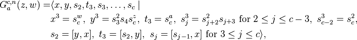
As a concrete example we take the metabelian -groups with bicyclic centre, which are represented by big full disks as vertices, of the coclass tree diagram in Figure 4.
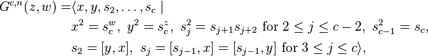
They form ten periodic infinite sequences, four, resp. six, for even, resp. odd, nilpotency class , and can be characterized with the aid of a parametrized polycyclic power-commutator presentation:
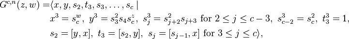
where  is the nilpotency class, with
  is the order, and
  ,
,  are parameters.
The transfer target type (TTT) of the group  depends only on the nilpotency class , is independent of the parameters
  , and is given uniformly by
.
This phenomenon is called a polarization, more precisely a uni-polarization,
[5]
at the first component.
, and is given uniformly by
.
This phenomenon is called a polarization, more precisely a uni-polarization,
[5]
at the first component.
The transfer kernel type (TKT) of the group is independent of the nilpotency class , but depends on the parameters , and is given by
c.18, , for  (a mainline group),
H.4, , for
(a mainline group),
H.4, , for  (two capable groups),
E.6, , for
(two capable groups),
E.6, , for  (a terminal group), and
E.14,
(a terminal group), and
E.14,  , for
, for  (two terminal groups).
For even nilpotency class, the two groups of types H.4 and E.14, which differ in the sign of the parameter
(two terminal groups).
For even nilpotency class, the two groups of types H.4 and E.14, which differ in the sign of the parameter  only, are isomorphic.
These statements can be deduced by means of the following considerations.
As a preparation, it is useful to compile a list of some commutator relations, starting with those given in the presentation,
 for
for  and
and  for
for  ,
which shows that the bicyclic centre is given by
,
which shows that the bicyclic centre is given by  .
By means of the right product rule
.
By means of the right product rule
 and the right power rule
 ,
we obtain
,
we obtain
 ,
,  , and
, and  , for
, for  .
.
The maximal subgroups of are taken in a similar way as in the section on the computational implementation, namely
 ,
,
 ,
,
 , and
, and
 .
.
Their derived subgroups are crucial for the behavior of the Artin transfers. By making use of the general formula  , where ,
and where we know that
, where ,
and where we know that  in the present situation,
it follows that
in the present situation,
it follows that
 ,
,
 ,
,
 , and
, and
 .
Note that
.
Note that  is not far from being abelian, since
  is contained in the centre .
As the first main result, we are now in the position to determine the abelian type invariants of the derived quotients:
 , the unique quotient which grows with increasing nilpotency class ,
since
, the unique quotient which grows with increasing nilpotency class ,
since  for even
  and
and  for odd
  ,
,
 ,
,
 ,
,
 ,
since generally
,
since generally  , but
, but  for
for  , whereas
  for
for  and
and  .
.
Now we come to the kernels of the Artin transfer homomorphisms . It suffices to investigate the induced transfers  and to begin by finding expressions for the images
  of elements
  , which can be expressed in the form
  with exponents
  . First, we exploit outer transfers as much as possible:

 ,
,

 ,
,
 and
and  , for
, for  .
Next, we treat the unavoidable inner transfers, which are more intricate. For this purpose, we use the polynomial identity
.
Next, we treat the unavoidable inner transfers, which are more intricate. For this purpose, we use the polynomial identity  to obtain:


 and
and

 .
Finally, we combine the results: generally
.
Finally, we combine the results: generally
 , and in particular,
 ,
,
 ,
,
 , for .
To determine the kernels, it remains to solve the following equations:
, for .
To determine the kernels, it remains to solve the following equations:
 arbitrary for ,
  with arbitrary for ,
  with arbitrary
  for , and
  for ,
furthermore,
for ,
furthermore,
 with arbitrary ,
 with arbitrary , for .
The following equivalences, for any
with arbitrary , for .
The following equivalences, for any  , finish the justification of the statements:
with arbitrary
, finish the justification of the statements:
with arbitrary 
 ,
with arbitrary
,
with arbitrary 
 ,
,

 ,
,

 , and
both arbitrary
, and
both arbitrary 
 .
Consequently, the last three components of the TKT are independent of the parameters , which means that both, the TTT and the TKT, reveal a uni-polarization at the first component.
.
Consequently, the last three components of the TKT are independent of the parameters , which means that both, the TTT and the TKT, reveal a uni-polarization at the first component.
Systematic library of SDTs
The aim of this section is to present a collection of structured coclass trees (SCTs) of finite p-groups with parametrized presentations and a succinct summary of invariants.
The underlying prime is restricted to small values  .
The trees are arranged according to increasing coclass
.
The trees are arranged according to increasing coclass  and different abelianizations within each coclass.
To keep the descendant numbers manageable, the trees are pruned by eliminating vertices of depth bigger than one.
Further, we omit trees where stabilization criteria enforce a common TKT of all vertices, since we do not consider such trees as structured any more.
The invariants listed include
and different abelianizations within each coclass.
To keep the descendant numbers manageable, the trees are pruned by eliminating vertices of depth bigger than one.
Further, we omit trees where stabilization criteria enforce a common TKT of all vertices, since we do not consider such trees as structured any more.
The invariants listed include
- pre-period and period length,
- depth and width of branches,
- uni-polarization, TTT and TKT,
- -groups.
We refrain from giving justifications for invariants, since the way how invariants are derived from presentations was demonstrated exemplarily in the section on commutator calculus
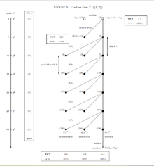
Coclass 1
For each prime , the unique tree of p-groups of maximal class is endowed with information on TTTs and TKTs, that is,  for ,
for ,  for , and
  for
for  . In the last case, the tree is restricted to metabelian -groups.
The -groups of coclass in Figure 5 can be defined by the following parametrized polycyclic pc-presentation, quite different from Blackburn's presentation.
[4]
where the nilpotency class is , the order is  with
with  , and are parameters.
The branches are strictly periodic with pre-period and period length , and have depth and width .
Polarization occurs for the third component and the TTT is
, and are parameters.
The branches are strictly periodic with pre-period and period length , and have depth and width .
Polarization occurs for the third component and the TTT is  , only dependent on and with cyclic
  .
The TKT depends on the parameters and is
.
The TKT depends on the parameters and is
 for the dihedral mainline vertices with ,
 for the terminal generalized quaternion groups with
  ,
and
,
and  for the terminal semi dihedral groups with .
There are two exceptions, the abelian root with
for the terminal semi dihedral groups with .
There are two exceptions, the abelian root with  and , and the usual quaternion group with
  and .
and .
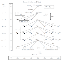
The -groups of coclass in Figure 6 can be defined by the following parametrized polycyclic pc-presentation, slightly different from Blackburn's presentation.
[4]
where the nilpotency class is , the order is with , and  are parameters.
The branches are strictly periodic with pre-period and period length , and have depth and width
are parameters.
The branches are strictly periodic with pre-period and period length , and have depth and width  .
Polarization occurs for the first component and the TTT is
.
Polarization occurs for the first component and the TTT is  , only dependent on and
  .
The TKT depends on the parameters and is
for the mainline vertices with
.
The TKT depends on the parameters and is
for the mainline vertices with 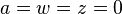 ,
,
 for the terminal vertices with
 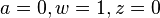 ,
for the terminal vertices with
,
for the terminal vertices with  ,
and for the terminal vertices with
,
and for the terminal vertices with  .
There exist three exceptions, the abelian root with
.
There exist three exceptions, the abelian root with  , the extra special group of exponent with
  and , and the Sylow -subgroup of the alternating group
  with
with  .
Mainline vertices and vertices on odd branches are -groups.
.
Mainline vertices and vertices on odd branches are -groups.
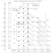
The metabelian -groups of coclass in Figure 7 can be defined by the following parametrized polycyclic pc-presentation, slightly different from Miech's presentation.
[15]
where the nilpotency class is , the order is  with , and are parameters.
The (metabelian!) branches are strictly periodic with pre-period and period length , and have depth and width
with , and are parameters.
The (metabelian!) branches are strictly periodic with pre-period and period length , and have depth and width  . (The branches of the complete tree, including non-metabelian groups, are only virtually periodic and have bounded width but unbounded depth!)
Polarization occurs for the first component and the TTT is
. (The branches of the complete tree, including non-metabelian groups, are only virtually periodic and have bounded width but unbounded depth!)
Polarization occurs for the first component and the TTT is  , only dependent on and the defect of commutativity
  .
The TKT depends on the parameters and is
.
The TKT depends on the parameters and is
 for the mainline vertices with ,
 for the terminal vertices with ,
 for the terminal vertices with
  ,
and for the vertices with
,
and for the vertices with  .
There exist three exceptions, the abelian root with
.
There exist three exceptions, the abelian root with  , the extra special group of exponent
  with
with  and
and  , and the group
  with
with  .
Mainline vertices and vertices on odd branches are -groups.
.
Mainline vertices and vertices on odd branches are -groups.
Coclass 2
Abelianization of type (p,p)
Three coclass trees,  ,
,  and
and  for , are endowed with information concerning TTTs and TKTs.
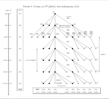
On the tree , the -groups of coclass with bicyclic centre in Figure 8 can be defined by the following parametrized polycyclic pc-presentation.
[5]
where the nilpotency class is , the order is with , and are parameters.
The branches are strictly periodic with pre-period and period length , and have depth and width  .
Polarization occurs for the first component and the TTT is
.
Polarization occurs for the first component and the TTT is  , only dependent on .
The TKT depends on the parameters and is
for the mainline vertices with ,
for the capable vertices with ,
for the terminal vertices with ,
and
, only dependent on .
The TKT depends on the parameters and is
for the mainline vertices with ,
for the capable vertices with ,
for the terminal vertices with ,
and  for the terminal vertices with .
Mainline vertices and vertices on even branches are -groups.
for the terminal vertices with .
Mainline vertices and vertices on even branches are -groups.
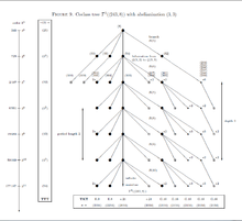
On the tree , the -groups of coclass with bicyclic centre in Figure 9 can be defined by the following parametrized polycyclic pc-presentation.
[5]
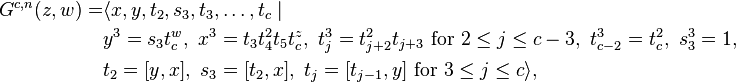
where the nilpotency class is  , the order is with , and are parameters.
The branches are strictly periodic with pre-period and period length , and have depth and width
, the order is with , and are parameters.
The branches are strictly periodic with pre-period and period length , and have depth and width  .
Polarization occurs for the second component and the TTT is
.
Polarization occurs for the second component and the TTT is  , only dependent on .
The TKT depends on the parameters and is
, only dependent on .
The TKT depends on the parameters and is
 for the mainline vertices with ,
 for the capable vertices with ,
 for the terminal vertices with ,
and
for the terminal vertices with ,
and  for the terminal vertices with .
Mainline vertices and vertices on even branches are -groups.
for the terminal vertices with .
Mainline vertices and vertices on even branches are -groups.
Abelianization of type (p2,p)
 and
and  for ,
for ,
 and
and  for .
for .
Abelianization of type (p,p,p)
 for , and
  for .
for .
Coclass 3
Abelianization of type (p2,p)
 ,
,  and
and  for .
for .
Abelianization of type (p,p,p)
 and
and  for ,
for ,
 and
and  for .
for .
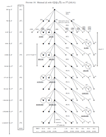
Arithmetical applications
In algebraic number theory and class field theory, structured descendant trees (SDTs) of finite p-groups provide an excellent tool for
- visualizing the location of various non-abelian p-groups
 associated with algebraic number fields ,
 - displaying additional information about the groups in labels attached to corresponding vertices, and
- emphasizing the periodicity of occurrences of the groups on branches of coclass trees.
- visualizing the location of various non-abelian p-groups
For instance, let be a prime number, and assume that
 denotes the second Hilbert p-class field of an algebraic number field ,
that is the maximal metabelian unramified extension of of degree a power of .
Then the second p-class group
denotes the second Hilbert p-class field of an algebraic number field ,
that is the maximal metabelian unramified extension of of degree a power of .
Then the second p-class group  of
is usually a non-abelian p-group of derived length and
frequently permits to draw conclusions about the entire p-class field tower of ,
that is the Galois group
of
is usually a non-abelian p-group of derived length and
frequently permits to draw conclusions about the entire p-class field tower of ,
that is the Galois group  of the maximal unramified pro-p extension
  of .
of .
Given a sequence of algebraic number fields with fixed signature  ,
ordered by the absolute values
,
ordered by the absolute values  of their discriminants
  ,
a suitable structured coclass tree (SCT)
,
a suitable structured coclass tree (SCT)  ,
or also the finite sporadic part
,
or also the finite sporadic part  of a coclass graph
  ,
whose vertices are entirely or partially realized
by second p-class groups
,
whose vertices are entirely or partially realized
by second p-class groups  of the fields
is endowed with additional arithmetical structure
when each realized vertex
of the fields
is endowed with additional arithmetical structure
when each realized vertex  , resp.
  , is mapped to
data concerning the fields such that
, is mapped to
data concerning the fields such that  .
.
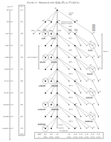
Example
To be specific, let and consider complex quadratic fields  with fixed signature
  having -class groups with type invariants .
See OEIS A242863 .
Their second -class groups
having -class groups with type invariants .
See OEIS A242863 .
Their second -class groups  have been determined by D. C. Mayer
[11]
for the range
have been determined by D. C. Mayer
[11]
for the range  ,
and, most recently, by N. Boston, M. R. Bush and F. Hajir
[16]
for the extended range
,
and, most recently, by N. Boston, M. R. Bush and F. Hajir
[16]
for the extended range  .
.
Let us firstly select the two structured coclass trees (SCTs)
and ,
which are known from Figures 8 and 9 already,
and endow these trees with additional arithmetical structure by
surrounding a realized vertex  with a circle and attaching an adjacent underlined boldface integer
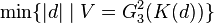 which gives the minimal absolute discriminant
such that is realized by the second -class group
which gives the minimal absolute discriminant
such that is realized by the second -class group  .
Then we obtain the arithmetically structured coclass trees (ASCTs) in Figures 10 and 11,
which, in particular, give an impression of the actual distribution of second -class groups.
[5]
See OEIS A242878 .
.
Then we obtain the arithmetically structured coclass trees (ASCTs) in Figures 10 and 11,
which, in particular, give an impression of the actual distribution of second -class groups.
[5]
See OEIS A242878 .
State  |
TKT E.14 |
TKT E.6 |
TKT H.4 |
TKT E.9 |
TKT E.8 |
TKT G.16 |
|---|---|---|---|---|---|---|
GS  |  |  |  |  |  |  |
ES1  |  |  |  |  |  |  |
ES2  |  |  |  |  |  |  |
ES3  |  |  |  |  |  |  |
ES4  |  |
Concerning the periodicity of occurrences of second -class groups of complex quadratic fields,
it was proved
[11]
that only every other branch of the trees in Figures 10 and 11 can be populated by these metabelian -groups and that
the distribution sets in with a ground state (GS) on branch
and continues with higher excited states (ES) on the branches  with even
  .
This periodicity phenomenon is underpinned by
three sequences with fixed TKTs
[10]
.
This periodicity phenomenon is underpinned by
three sequences with fixed TKTs
[10]
on the ASCT ,
and by three sequences with fixed TKTs
[10]
on the ASCT .
Up to now,
[16]
the ground state and three excited states are known for each of the six sequences,
and for TKT E.9 even the fourth excited state occurred already.
The minimal absolute discriminants of the various states of each of the six periodic sequences are presented in Table 2.
Data for the ground states (GS) and the first excited states (ES1) has been taken from D. C. Mayer,
[11]
most recent information on the second, third and fourth excited states (ES2, ES3, ES4) is due to N. Boston, M. R. Bush and F. Hajir.
[16]
| < |
Total  |
TKT D.10    |
TKT D.5  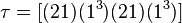 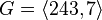 |
TKT H.4  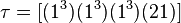 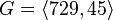 |
TKT G.19    |
|---|---|---|---|---|---|
 |  |  |  |  |  |
 |  |  |  |  |  |
 |  |  |  |  |  |
In contrast, let us secondly select the sporadic part  of the coclass graph for demonstrating that
another way of attaching additional arithmetical structure to descendant trees is to display the counter
of the coclass graph for demonstrating that
another way of attaching additional arithmetical structure to descendant trees is to display the counter
 of hits of a realized vertex by the second -class group
of fields with absolute discriminants below a given upper bound
of hits of a realized vertex by the second -class group
of fields with absolute discriminants below a given upper bound  , for instance .
With respect to the total counter of all complex quadratic fields
with -class group of type and discriminant
, for instance .
With respect to the total counter of all complex quadratic fields
with -class group of type and discriminant  ,
this gives the relative frequency as an approximation to the asymptotic density of the population
in Figure 12 and Table 3.
Exactly four vertices of the finite sporadic part of
are populated by second -class groups :
,
this gives the relative frequency as an approximation to the asymptotic density of the population
in Figure 12 and Table 3.
Exactly four vertices of the finite sporadic part of
are populated by second -class groups :
 , OEIS A247689
  , OEIS A247690
  , OEIS A242873
  , OEIS A247688
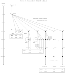
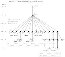
Comparison of various primes
Now let  and consider complex quadratic fields with fixed signature
and p-class groups of type .
The dominant part of the second p-class groups of these fields
populates the top vertices of order
and consider complex quadratic fields with fixed signature
and p-class groups of type .
The dominant part of the second p-class groups of these fields
populates the top vertices of order  of the sporadic part
  of the coclass graph
  ,
which belong to the stem of P. Hall's isoclinism family
,
which belong to the stem of P. Hall's isoclinism family  ,
or their immediate descendants of order
,
or their immediate descendants of order  .
For primes
.
For primes  , the stem of consists of
  regular p-groups
and reveals a rather uniform behaviour with respect to TKTs and TTTs,
but the seven -groups in the stem of are irregular.
We emphasize that there also exist several ( for and for )
infinitely capable vertices in the stem of
which are partially roots of coclass trees.
However, here we focus on the sporadic vertices
which are either isolated Schur -groups ( for and for )
or roots of finite trees within ( for each ).
For , the TKT of Schur -groups is a permutation
whose cycle decomposition does not contain transpositions,
whereas the TKT of roots of finite trees
is a compositum of disjoint transpositions
having an even number ( or ) of fixed points.
regular p-groups
and reveals a rather uniform behaviour with respect to TKTs and TTTs,
but the seven -groups in the stem of are irregular.
We emphasize that there also exist several ( for and for )
infinitely capable vertices in the stem of
which are partially roots of coclass trees.
However, here we focus on the sporadic vertices
which are either isolated Schur -groups ( for and for )
or roots of finite trees within ( for each ).
For , the TKT of Schur -groups is a permutation
whose cycle decomposition does not contain transpositions,
whereas the TKT of roots of finite trees
is a compositum of disjoint transpositions
having an even number ( or ) of fixed points.
We endow the forest (a finite union of descendant trees)
with additional arithmetical structure
by attaching the minimal absolute discriminant  to each realized vertex
  .
The resulting structured sporadic coclass graph is shown in Figure 13 for , in Figure 14 for ,
and in Figure 15 for
.
The resulting structured sporadic coclass graph is shown in Figure 13 for , in Figure 14 for ,
and in Figure 15 for  .
.
References
- ↑ 1.0 1.1 Huppert, B. (1979). Endliche Gruppen I. Grundlehren der mathematischen Wissenschaften, Vol. 134, Springer-Verlag Berlin Heidelberg New York.
- ↑ 2.0 2.1 Schur, I. (1902). "Neuer Beweis eines Satzes über endliche Gruppen". Sitzungsb. Preuss. Akad. Wiss.: 1013–1019.
- ↑ 3.0 3.1 Artin, E. (1929). "Idealklassen in Oberkörpern und allgemeines Reziprozitätsgesetz". Abh. Math. Sem. Univ. Hamburg 7: 46–51.
- ↑ 4.0 4.1 4.2 Blackburn, N. (1958). "On a special class of p-groups". Acta Math. 100: 45–92. doi:10.1007/bf02559602.
- ↑ 5.0 5.1 5.2 5.3 5.4 5.5 Mayer, D. C. (2013). "The distribution of second p-class groups on coclass graphs". J. Théor. Nombres Bordeaux 25 (2): 401–456. doi:10.5802/jtnb.842.
- ↑ Chang, S. M., Foote, R. (1980). "Capitulation in class field extensions of type (p,p)". Can. J. Math. 32 (5): 1229–1243. doi:10.4153/cjm-1980-091-9.
- ↑ Besche, H. U., Eick, B., O'Brien, E. A. (2005). The SmallGroups Library – a library of groups of small order. An accepted and refereed GAP 4 package, available also in MAGMA.
- ↑ Besche, H. U., Eick, B., O'Brien, E. A. (2002). "A millennium project: constructing small groups". Int. J. Algebra Comput. 12: 623–644. doi:10.1142/s0218196702001115.
- ↑ 9.0 9.1 9.2 9.3 Bush, M. R., Mayer, D. C. (2015). "3-class field towers of exact length 3". J. Number Theory 147: 766–777 (preprint: arXiv:1312.0251 [math.NT], 2013). doi:10.1016/j.jnt.2014.08.010.
- ↑ 10.0 10.1 10.2 10.3 10.4 Mayer, D. C. (2012). "Transfers of metabelian p-groups". Monatsh. Math. 166 (3-4): 467–495. doi:10.1007/s00605-010-0277-x.
- ↑ 11.0 11.1 11.2 11.3 11.4 11.5 11.6 Mayer, D. C. (2012). "The second p-class group of a number field". Int. J. Number Theory 8 (2): 471–505. doi:10.1142/s179304211250025x.
- ↑ Scholz, A., Taussky, O. (1934). "Die Hauptideale der kubischen Klassenkörper imaginär quadratischer Zahlkörper: ihre rechnerische Bestimmung und ihr Einfluß auf den Klassenkörperturm". J. Reine Angew. Math. 171: 19–41.
- ↑ Newman, M. F. (1977). Determination of groups of prime-power order. pp. 73-84, in: Group Theory, Canberra, 1975, Lecture Notes in Math., Vol. 573, Springer, Berlin.
- ↑ O'Brien, E. A. (1990). "The p-group generation algorithm". J. Symbolic Comput. 9: 677–698. doi:10.1016/s0747-7171(08)80082-x.
- ↑ Miech, R. J. (1970). "Metabelian p-groups of maximal class". Trans. Amer. Math. Soc. 152: 331–373. doi:10.1090/s0002-9947-1970-0276343-7.
- ↑ 16.0 16.1 16.2 Boston, N., Bush, M. R., Hajir, F. (2013). "Heuristics for p-class towers of imaginary quadratic fields". Math. Ann.: (preprint: arXiv:1111.4679v1 [math.NT], 2011).