Arithmetic–geometric mean

In mathematics, the arithmetic–geometric mean (AGM) of two positive real numbers $x$ and $y$ is defined as follows:

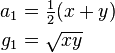
First compute the arithmetic mean of $x$ and $y$ and call it $a 1$ . Next compute the geometric mean of $x$ and $y$ and call it $g 1$ ; this is the square root of the product $xy$ :

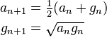
\begin{align} a_1 &= \tfrac12(x + y)\\ g_1 &= \sqrt{xy} \end{align}

Then iterate this operation with $a 1$ taking the place of $x$ and $g 1$ taking the place of $y$ . In this way, two sequences $(a n)$ and $(g n)$ are defined:

\begin{align} a_{n+1} &= \tfrac12(a_n + g_n)\\ g_{n+1} &= \sqrt{a_n g_n} \end{align}

These two sequences converge to the same number, which is the arithmetic–geometric mean of $x$ and $y$ ; it is denoted by $M (x, y)$ , or sometimes by $agm(x, y)$ .

This can be used for algorithmic purposes as in the AGM method.

Example

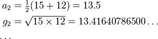
To find the arithmetic–geometric mean of $a 0 = 24$ and $g 0 = 6$ , first calculate their arithmetic mean and geometric mean, thus:

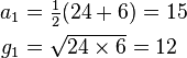
\begin{align} a_1 &= \tfrac12(24 + 6) = 15\\ g_1 &= \sqrt{24 \times 6} = 12 \end{align}

and then iterate as follows:

\begin{align} a_2 &= \tfrac12(15 + 12) = 13.5\\ g_2 &= \sqrt{15 \times 12} = 13.41640786500\dots\\ \dots \end{align}

The first five iterations give the following values:

$n$	$a n$	$g n$
0	24	6
1	15	12
2	13.5	13.416407864998738178455042…
3	13.458203932499369089227521…	13.458139030990984877207090…
4	13.458171481745176983217305…	13.458171481706053858316334…
5	13.458171481725615420766820…	13.458171481725615420766806…

As can be seen, the number of digits in agreement (underlined) approximately doubles with each iteration. The arithmetic–geometric mean of 24 and 6 is the common limit of these two sequences, which is approximately 13.4581714817256154207668131569743992430538388544.^[1]

History

The first algorithm based on this sequence pair appeared in the works of Lagrange. Its properties were further analyzed by Gauss.^[2]

Properties

The geometric mean of two positive numbers is never bigger than the arithmetic mean (see inequality of arithmetic and geometric means); as a consequence, $(g n)$ is an increasing sequence, $(a n)$ is a decreasing sequence, and $g n \leq M (x, y) \leq a n$ . These are strict inequalities if $x \neq y$ .

$M (x, y)$ is thus a number between the geometric and arithmetic mean of $x$ and $y$ ; in particular it is between $x$ and $y$ .

If $r \geq 0$ , then $M (rx, ry) = r M (x, y)$ .

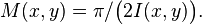
There is an integral-form expression for $M (x, y)$ :

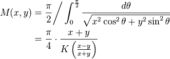
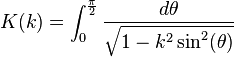
\begin{align} M(x,y) &= \frac\pi2\bigg/\int_0^\frac{\pi}{2}\frac{d\theta}{\sqrt{x^2\cos^2\theta+y^2\sin^2\theta}}\\ &=\frac{\pi}{4} \cdot \frac{x + y}{K\left( \frac{x - y}{x + y} \right)} \end{align}

where $K (k)$ is the complete elliptic integral of the first kind:

K(k) = \int_0^\frac{\pi}{2}\frac{d\theta}{\sqrt{1 - k^2\sin^2(\theta)}}

Indeed, since the arithmetic–geometric process converges so quickly, it provides an effective way to compute elliptic integrals via this formula. In engineering, it is used for instance in elliptic filter design.^[3]

Related concepts

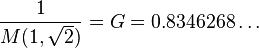
The reciprocal of the arithmetic–geometric mean of 1 and the square root of 2 is called Gauss's constant, after Carl Friedrich Gauss.

\frac{1}{M(1, \sqrt{2})} = G = 0.8346268\dots

The geometric–harmonic mean can be calculated by an analogous method, using sequences of geometric and harmonic means. The arithmetic–harmonic mean can be similarly defined, but takes the same value as the geometric mean.

The arithmetic–geometric mean can be used to compute logarithms and complete elliptic integrals of the first kind. A modified arithmetic–geometric mean can be used to efficiently compute complete elliptic integrals of the second kind.^[4]

Proof of existence

From inequality of arithmetic and geometric means we can conclude that:

g_n \leqslant a_n

and thus

g_{n + 1} = \sqrt{g_n \cdot a_n} \geqslant \sqrt{g_n \cdot g_n} = g_n

that is, the sequence $g n$ is nondecreasing.

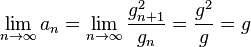
Furthermore, it is easy to see that it is also bounded above by the larger of $x$ and $y$ (which follows from the fact that both arithmetic and geometric means of two numbers both lie between them). Thus by the monotone convergence theorem the sequence is convergent, so there exists a $g$ such that:

\lim_{n\to \infty}g_n = g

However, we can also see that:

a_n = \frac{g_{n + 1}^2}{g_n}

and so:

\lim_{n\to \infty}a_n = \lim_{n\to \infty}\frac{g_{n + 1}^2}{g_{n}} = \frac{g^2}{g} = g

Q.E.D.

Proof of the integral-form expression

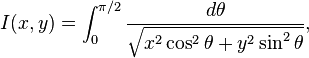
This proof is given by Gauss.^[2] Let

I(x,y) = \int_0^{\pi/2}\frac{d\theta}{\sqrt{x^2\cos^2\theta+y^2\sin^2\theta}},

Changing the variable of integration to $\theta'$ , where

\sin\theta = \frac{2x\sin\theta'}{(x+y)+(x-y)\sin^2\theta'},

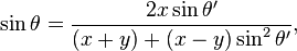
gives

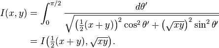
\begin{align} I(x,y) &= \int_0^{\pi/2}\frac{d\theta'}{\sqrt{\bigl(\frac12(x+y)\bigr)^2\cos^2\theta'+\bigl(\sqrt{xy}\bigr)^2\sin^2\theta'}}\\ &= I\bigl(\tfrac12(x+y),\sqrt{xy}\bigr). \end{align}

Thus, we have

\begin{align} I(x,y) &= I(a_1, g_1) = I(a_2, g_2) = \cdots\\ &= I\bigl(M(x,y),M(x,y)\bigr) = \pi/\bigr(2M(x,y)\bigl). \end{align}

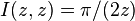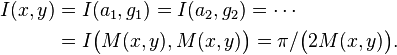
The last equality comes from observing that $I(z,z) = \pi/(2z)$ .

Finally, we obtain the desired result

M(x,y) = \pi/\bigl(2 I(x,y) \bigr).

External links

References

Adlaj, Semjon (September 2012). "An eloquent formula for the perimeter of an ellipse" (PDF). Notices of the AMS 59 (8): 1094–1099. doi:10.1090/noti879.
Jonathan Borwein, Peter Borwein, Pi and the AGM. A study in analytic number theory and computational complexity. Reprint of the 1987 original. Canadian Mathematical Society Series of Monographs and Advanced Texts, 4. A Wiley-Interscience Publication. John Wiley & Sons, Inc., New York, 1998. xvi+414 pp. ISBN 0-471-31515-X MR 1641658
Zoltán Daróczy, Zsolt Páles, Gauss-composition of means and the solution of the Matkowski–Suto problem. Publ. Math. Debrecen 61/1-2 (2002), 157–218.
M. Hazewinkel (2001), "Arithmetic–geometric mean process", in Hazewinkel, Michiel, Encyclopedia of Mathematics, Springer, ISBN 978-1-55608-010-4
Weisstein, Eric W., "Arithmetic–Geometric mean", MathWorld.

↑ agm(24, 6) at WolframAlpha
↑ 2.0 2.1 David A. Cox (2004). "The Arithmetic-Geometric Mean of Gauss". In J.L. Berggren, Jonathan M. Borwein, Peter Borwein. Pi: A Source Book. Springer. p. 481. ISBN 978-0-387-20571-7. first published in L'Enseignement Mathématique, t. 30 (1984), p. 275-330
↑ Hercules G. Dimopoulos (2011). Analog Electronic Filters: Theory, Design and Synthesis. Springer. pp. 147–155. ISBN 978-94-007-2189-0.
↑ Adlaj, Semjon (September 2012), "An eloquent formula for the perimeter of an ellipse" (PDF), Notices of the AMS 59 (8): 1094–1099, doi:10.1090/noti879, retrieved 2013-12-14