Activity coefficient
An activity coefficient is a factor used in thermodynamics to account for deviations from ideal behaviour in a mixture of chemical substances.[1] In an ideal mixture, the microscopic interactions between each pair of chemical species are the same (or macroscopically equivalent, the enthalpy change of solution and volume variation in mixing is zero) and, as a result, properties of the mixtures can be expressed directly in terms of simple concentrations or partial pressures of the substances present e.g. Raoult's law. Deviations from ideality are accommodated by modifying the concentration by an activity coefficient. Analogously, expressions involving gases can be adjusted for non-ideality by scaling partial pressures by a fugacity coefficient.
The concept of activity coefficient is closely linked to that of activity in chemistry.
Thermodynamic definition
The chemical potential,  , of a substance B in an ideal mixture of liquids or an ideal solution is given by

where  is the chemical potential in the standard state and xB is the mole fraction of the substance in the mixture.
This is generalised to include non-ideal behavior by writing
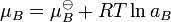
when  is the activity of the substance in the mixture with

where  is the activity coefficient, which may itself depend on
  . As approaches 1, the substance behaves as if it were ideal. For instance, if
  , then Raoult's law is accurate. For
  and
and  , substance B shows positive and negative deviation from Raoult's law, respectively. A positive deviation implies that substance B is more volatile.
In many cases, as goes to zero, the activity coefficient of substance B approaches a constant; this relationship is Henry's law for the solvent. These relationships are related to each other through the Gibbs–Duhem equation.[2]
Note that in general activity coefficients are dimensionless.
Modifying mole fractions or concentrations by activity coefficients gives the effective activities of the components, and hence allows expressions such as Raoult's law and equilibrium constants to be applied to both ideal and non-ideal mixtures.
Knowledge of activity coefficients is particularly important in the context of electrochemistry since the behaviour of electrolyte solutions is often far from ideal, due to the effects of the ionic atmosphere. Additionally, they are particularly important in the context of soil chemistry due to the low volumes of solvent and, consequently, the high concentration of electrolytes.[3]
Experimental determination of activity coefficients
Activity coefficients may be determined experimentally by making measurements on non-ideal mixtures. Use may be made of Raoult's law or Henry's law to provide a value for an ideal mixture against which the experimental value may be compared to obtain the activity coefficient. Other colligative properties, such as osmotic pressure may also be used.
For solution of substances which ionize in solution the activity coefficients of the cation and anion cannot be experimentally determined independently of each other because solution properties depend on both ions. In this case a mean activity coefficient,  , must be used. For a 1:1 electrolyte, such as NaCl it is defined as follows.

where γ+ and γ- are the activity coefficients of the cation and anion respectively.
More generally,The mean activity coefficient of a compound of formula ApBq is given by[4]
![\gamma_\pm=\sqrt[p+q]{\gamma_A^p\gamma_B^q}](../I/m/38e56041b9230a819b7f0895a2089928.png)
Single-ion activity coefficients can be calculated theoretically, for example by using the Debye–Hückel equation. The theoretical equation can be tested by combining the calculated single-ion activity coefficients to give mean values which can be compared to experimental values.
Theoretical calculation of activity coefficients
Activity coefficients of electrolyte solutions may be calculated theoretically, using the Debye–Hückel equation or extensions such as the Davies equation,[5] Pitzer equations[6] or TCPC model.[7][8][9][10] Specific ion interaction theory (SIT)[11] may also be used.
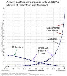
For non-electrolyte solutions correlative methods such as UNIQUAC, NRTL, MOSCED or UNIFAC may be employed, provided fitted component-specific or model parameters are available. COSMO-RS is a theoretical method which is less dependent on model parameters as required information is obtained from quantum mechanics calculations specific to each molecule (sigma profiles) combined with a statistical thermodynamics treatment of surface segments.[12]
For uncharged species, the activity coefficient γ0 mostly follows a salting-out model:[13]

This simple model predicts activities of many species (dissolved undissociated gases such as CO2, H2S, NH3, undissociated acids and bases) to high ionic strengths (up to 5 mol/kg). The value of the constant b for CO2 is 0.11 at 10 °C and 0.20 at 330 °C.[14][15]
For water (solvent), the activity aw can be calculated using:[13]
 φ
φ
where ν is the number of ions produced from the dissociation of one molecule of the dissolved salt, m is the molality of the salt dissolved in water, φ is the osmotic coefficient of water, and the constant 55.51 represents the molality of water. In the above equation, the activity of a solvent (here water) is represented as inversely proportional to the number of particles of salt versus that of the solvent.
Link to ionic diameter
The ionic activity coefficient is connected to the ionic diameter a by the formula:
where A and B are constant, zi is the valence number of the ion, and I is ionic strength.
Dependence on state parameters
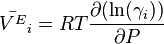
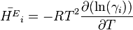
The derivative of the activity coefficient to temperature and respectively pressure are connected to the excess molar quantities.
Application to chemical equilibrium
At equilibrium, the sum of the chemical potentials of the reactants is equal to the sum of the chemical potentials of the products. The Gibbs free energy change for the reactions,  , is equal to the difference between these sums and therefore, at equilibrium, is equal to zero. Thus, for an equilibrium such as


Substitute in the expressions for the chemical potential of each reactant:

Upon rearrangement this expression becomes
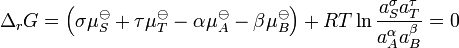
The sum 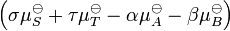 is the standard free energy change for the reaction,
  . Therefore

K is the equilibrium constant. Note that activities and equilibrium constants are dimensionless numbers.
This derivation serves two purposes. It shows the relationship between standard free energy change and equilibrium constant. It also shows that an equilibrium constant is defined as a quotient of activities. In practical terms this is inconvenient. When each activity is replaced by the product of a concentration and an activity coefficient, the equilibrium constant is defined as
![K= \frac{[S]^\sigma[T]^\tau}{[A]^\alpha[B]^\beta} \times \frac{\gamma_S^\sigma \gamma_T^\tau}{\gamma_A^\alpha \gamma_B^\beta}](../I/m/48b1a5305731008ed0b72d58a9184efc.png)
where [S] denotes the concentration of S, etc. In practice equilibrium constants are determined in a medium such that the quotient of activity coefficient is constant and can be ignored, leading to the usual expression
![K= \frac{[S]^\sigma[T]^\tau}{[A]^\alpha[B]^\beta}](../I/m/eef75b6fdacc80806a69add59e6f4110.png)
which applies under the conditions that the activity quotient has a particular (constant) value.
References
- ↑ IUPAC, Compendium of Chemical Terminology, 2nd ed. (the "Gold Book") (1997). Online corrected version: (2006–) "Activity coefficient".
- ↑ R. DeHoff, Thermodynamic in Materials Science, Taylor and Francis, 2006. pp230-1
- ↑ Jorge G. Ibanez; Margarita Hernandez-Esparza; Carmen Doria-Serrano; Mono Mohan Singh (2007). Environmental Chemistry: Fundamentals. Springer. ISBN 978-0-387-26061-7.
- ↑ Atkins, Peter; dePaula, Julio (2006). "Section 5.9, The activities of ions in solution". Physical Chemisrry (8th ed.). OUP. ISBN 9780198700722.
- ↑ C. W. Davies, Ion Association, Butterworths, 1962
- ↑ I. Grenthe and H. Wanner, Guidelines for the extrapolation to zero ionic strength, http://www.nea.fr/html/dbtdb/guidelines/tdb2.pdf
- ↑ X. Ge, X. Wang, M. Zhang, S. Seetharaman. Correlation and Prediction of Activity and Osmotic Coefficients of Aqueous Electrolytes at 298.15 K by the Modified TCPC Model. J. Chem. Eng. Data. 52 (2007) 538-547.http://pubs.acs.org/doi/abs/10.1021/je060451k
- ↑ X. Ge, M. Zhang, M. Guo, X. Wang, Correlation and Prediction of Thermodynamic Properties of Non-aqueous Electrolytes by the Modified TCPC Model. J. Chem. Eng. Data. 53 (2008)149-159.http://pubs.acs.org/doi/abs/10.1021/je700446q
- ↑ X. Ge, M. Zhang, M. Guo, X. Wang. Correlation and Prediction of thermodynamic properties of Some Complex Aqueous Electrolytes by the Modified Three-Characteristic-Parameter Correlation Model. J. Chem. Eng. Data. 53 (2008) 950-958.http://pubs.acs.org/doi/abs/10.1021/je7006499
- ↑ X. Ge, X. Wang. A Simple Two-Parameter Correlation Model for Aqueous Electrolyte across a wide range of temperature. J. Chem. Eng. Data. 54(2009)179-186.http://pubs.acs.org/doi/abs/10.1021/je800483q
- ↑ "Project: Ionic Strength Corrections for Stability Constants". IUPAC. Archived from the original on 29 October 2008. Retrieved 2008-11-15.
- ↑ Andreas Klamt, COSMO-RS: From Quantum Chemistry to Fluid Phase Thermodynamics and Drug Design, Elsevier, 2005.
- ↑ 13.0 13.1 J. N. Butler, Ionic Equilibrium, John Wiley and Sons, Inc., 1998.
- ↑ A. J. Elis and R. M. Golding, Am. J. Sci, 162, p 47-60, 1963.
- ↑ S. D. Malinin, Geokhimiya, 3, p. 235-245, 1959.
External links
- AIOMFAC online-model An interactive group-contribution model for the calculation of activity coefficients in organic-inorganic mixtures.
- Electrochimica Acta Single-ion activity coefficients