(a,b,0) class of distributions
In probability theory, the distribution of a discrete random variable  is said to be a member of the (a, b, 0) class of distributions if its probability mass function obeys
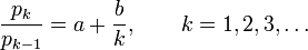
where 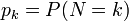 (provided
  and
and  exist and are real).
There are only three discrete distributions that satisfy the full form of this relationship: the Poisson, binomial and negative binomial distributions. These are also the three discrete distributions among the six members of the natural exponential family with quadratic variance functions (NEF–QVF).
More general distributions can be defined by fixing some initial values of pj and applying the recursion to define subsequent values. This can be of use in fitting distributions to empirical data. However, some further well-known distributions are available if the recursion above need only hold for a restricted range of values of k:[1] for example the logarithmic distribution and the discrete uniform distribution.
The (a, b, 0) class of distributions has important applications in actuarial science in the context of loss models.[2]
Properties
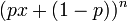
Sundt[3] proved that only the binomial distribution, the Poisson distribution and the negative binomial distribution belong to this class of distributions, with each distribution being represented by a different sign of a. The more usual parameters of these distributions are determined by both a and b. The properties of these distributions in relation to the present class of distributions are summarised in the following table. Note that  denotes the probability generating function.
| Distribution | ![P[N=k]\,](../I/m/7317e2df756bdb14b9035df9d192520e.png) |
 |
 |
 |
|
![E[N]\,](../I/m/488bf69dd760c64ad81a55dca2f3cf36.png) |
 |
|---|---|---|---|---|---|---|---|
| Binomial | 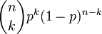 |
 |
 |
 |
 |
 |
 |
| Poisson |  |
 |
 |
 |
 |
|
|
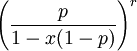
| Negative binomial | 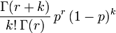 |
 |
 |
 |
 |
 |
 |
Plotting
An easy way to quickly determine whether a given sample was taken from a distribution from the (a,b,0) class is by graphing the ratio of two consecutive observed data (multiplied by a constant) against the x-axis.
By multiplying both sides of the recursive formula by  , you get
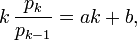
which shows that the left side is obviously a linear function of . When using a sample of  data, an approximation of the
  's need to be done. If
  represents the number of observations having the value , then
  is an unbiased estimator of the true .
Therefore, if a linear trend is seen, then it can be assumed that the data is taken from an (a,b,0) distribution. Moreover, the slope of the function would be the parameter , while the ordinate at the origin would be .
See also
References
- ↑ Hess, Klaus Th.; Liewald, Anett; Schmidt, Klaus D. (2002). "An extension of Panjer's recursion" (PDF). ASTIN Bulletin 32 (2): 283–297. doi:10.2143/AST.32.2.1030. Archived from the original on 2009-06-20. Retrieved 2009-06-18.
- ↑ Klugman, Stuart; Panjer, Harry; Gordon, Willmot (2004). Loss Models: From Data to Decisions. Series in Probability and Statistics (2nd ed.). New Jersey: Wiley. ISBN 0-471-21577-5.
- ↑ Sundt, Bjørn; Jewell, William S. (1981). "Further results on recursive evaluation of compound distributions" (PDF). ASTIN Bulletin (International Actuarial Association) 12 (1): 27–39.