Yeoh (hyperelastic model)
The Yeoh hyperelastic material model[1] is a phenomenological model for the deformation of nearly incompressible, nonlinear elastic materials such as rubber. The model is based on Ronald Rivlin's observation that the elastic properties of rubber may be described using a strain energy density function which is a power series in the strain invariants  .[2] The Yeoh model for incompressible rubber is a function only of
  . For compressible rubbers, a dependence on
  is added on. Since a polynomial form of the strain energy density function is used but all the three invariants of the left Cauchy-Green deformation tensor are not, the Yeoh model is also called the reduced polynomial model.
Yeoh model for incompressible rubbers
Strain energy density function
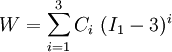
The original model proposed by Yeoh had a cubic form with only dependence and is applicable to purely incompressible materials. The strain energy density for this model is written as
where  are material constants. The quantity
  can be interpreted as the initial shear modulus.
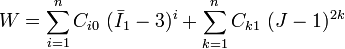
Today a slightly more generalized version of the Yeoh model is used.[3] This model includes  terms and is written as

When  the Yeoh model reduces to the neo-Hookean model for incompressible materials.
For consistency with linear elasticity the Yeoh model has to satisfy the condition
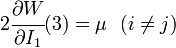
where  is the shear modulus of the material.
Now, at
is the shear modulus of the material.
Now, at  ,
,

Therefore, the consistency condition for the Yeoh model is

Stress-deformation relations
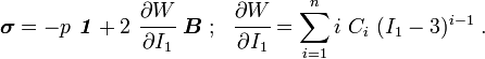
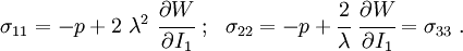
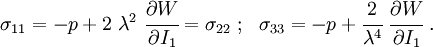
The Cauchy stress for the incompressible Yeoh model is given by
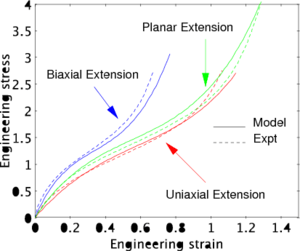
Uniaxial extension
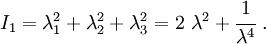
For uniaxial extension in the  -direction, the principal stretches are
  . From incompressibility
  . Hence
  .
Therefore,
.
Therefore,
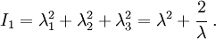
The left Cauchy-Green deformation tensor can then be expressed as

If the directions of the principal stretches are oriented with the coordinate basis vectors, we have
Since 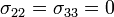 , we have
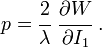
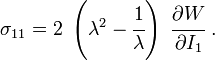
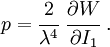
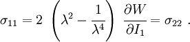
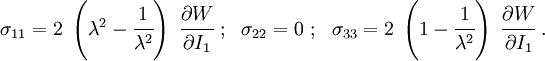
Therefore,
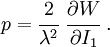
The engineering strain is  . The engineering stress is

Equibiaxial extension
For equibiaxial extension in the and  directions, the principal stretches are
  . From incompressibility . Hence
  .
Therefore,
.
Therefore,
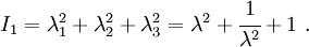
The left Cauchy-Green deformation tensor can then be expressed as

If the directions of the principal stretches are oriented with the coordinate basis vectors, we have
Since  , we have
Therefore,
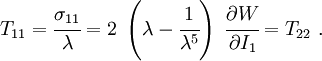
The engineering strain is . The engineering stress is
Planar extension
Planar extension tests are carried out on thin specimens which are constrained from deforming in one direction. For planar extension in the directions with the  direction constrained, the principal stretches are
  . From incompressibility . Hence
  .
Therefore,
.
Therefore,
The left Cauchy-Green deformation tensor can then be expressed as

If the directions of the principal stretches are oriented with the coordinate basis vectors, we have

Since  , we have
Therefore,
The engineering strain is . The engineering stress is

Yeoh model for compressible rubbers
A version of the Yeoh model that includes  dependence is used for compressible rubbers. The strain energy density function for this model is written as
where  , and
, and  are material constants. The quantity
  is interpreted as half the initial shear modulus, while
  is interpreted as half the initial bulk modulus.
When the compressible Yeoh model reduces to the neo-Hookean model for incompressible materials.
References
- ↑ Yeoh, O. H., 1993, "Some forms of the strain energy function for rubber," Rubber Chemistry and technology, Volume 66, Issue 5, November 1993, Pages 754-771.
- ↑ Rivlin, R. S., 1948, "Some applications of elasticity theory to rubber engineering", in Collected Papers of R. S. Rivlin vol. 1 and 2, Springer, 1997.
- ↑ Selvadurai, A. P. S., 2006, "Deflections of a rubber membrane", Journal of the Mechanics and Physics of Solids, vol. 54, no. 6, pp. 1093-1119.
See also
- Hyperelastic material
- Strain energy density function
- Mooney-Rivlin solid
- Finite strain theory
- Stress measures