Xenakis distribution
Probability density function | |
Cumulative distribution function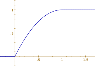 | |
| Parameters |  length of the interval (real) length of the interval (real) |
|---|---|
| Support | ![x\in [0;a]](/2014-wikipedia_en_all_02_2014/I/media/7/4/a/3/74a38b5620513e7232cc39b1e3b87b4f.png) |
 pour ![\scriptstyle x\in [0,a]](/2014-wikipedia_en_all_02_2014/I/media/a/7/2/5/a725b47e7479c1f38ac4b00a0c18b96b.png) | |
| CDF |  for for |
| Mean | ![\operatorname {E}[X]={\frac {a}{3}}](/2014-wikipedia_en_all_02_2014/I/media/b/b/2/c/bb2c9dd15896becd6cb720e790e3c65f.png) |
| Median | 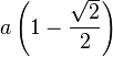 |
| Mode |  |
| Variance |  |
| Skewness |  |
| Ex. kurtosis |  |
| Entropy |  |
| MGF |  |
| CF |  |
In probability theory, a Xenakis distribution is a probability distribution the graph of whose probability density function on the interval from 0 to a positive number a is a straight line giving the function the value 0 at a. Thus the region under the graph of the density function is a triangle. It is a triangular distribution with parameters 0, a, and 0. It is named after Iannis Xenakis, who used this distribution in his book Musiques formelles (Formal Music),[1] where he described it as the distribution of the length of a line segment that is included inside another fixed line segment.

Properties
Probability density function
The probability density function of a Xenakis distribution is a linear function on ![[0,a]](/2014-wikipedia_en_all_02_2014/I/media/1/3/5/9/13596d6674a86fdafa24c4c414033e58.png) . Then, as a line segment is symmetric, its median is
. Then, as a line segment is symmetric, its median is  .
.
Cumulative distribution function
The cumulative distribution function of a Xenakis distribution is of degree 2; then, to simulate it with the use of the cumulative distribution function, one needs a square root.
Xenakis distribution of parameter 1

When its parameter is 1, a Xenakis distribution is a Beta distribution which parameters are 1 and 2. Hence, a Xenakis variable of parameter 1 can be defined also as the minimum of two variables which are uniform on ![[0,1]](/2014-wikipedia_en_all_02_2014/I/media/c/c/f/c/ccfcd347d0bf65dc77afe01a3306a96b.png)
Related distributions
- The minimum of 2 Xenakis variables of parameter 1 is Beta with parameters 1 and 4.
Simulation
Three algorithms are in use when simulating a Xenakis variable of parameter 1:
- The first version uses the definition: Generate 2 uniform random variables then compute the absolute value of their difference;
- A variant is suggested by the definition as a Beta variable: Generate 2 uniform variables then compute their minimum;
- Xenakis used the inverse of the cumulative distribution: The third version below.
Python (language)'s timeit module allows to measure the performances of these algorithms then to compare them:
from timeit import *
from random import *
from math import *

def version1():
	return abs(uniform(0,1)-uniform(0,1))
def version2():
	return min(uniform(0,1),uniform(0,1))
def version3():
	return 1-sqrt(1-uniform(0,1))

print(Timer('x=version1()',"from __main__ import version1").timeit())
print(Timer('x=version2()',"from __main__ import version2").timeit())
print(Timer('x=version3()',"from __main__ import version3").timeit())
Surprisingly, the third version is faster than the others, probably because it is the only one to use only one random uniform variable. It is even possible to make it faster with
def version3():
	return 1-sqrt(uniform(0,1))