Turbo code
In information theory, turbo codes (originally in French Turbocodes) are a class of high-performance forward error correction (FEC) codes developed in 1993, which were the first practical codes to closely approach the channel capacity, a theoretical maximum for the code rate at which reliable communication is still possible given a specific noise level. Turbo codes are finding use in 3G mobile communications and (deep space) satellite communications as well as other applications where designers seek to achieve reliable information transfer over bandwidth- or latency-constrained communication links in the presence of data-corrupting noise. Turbo codes are nowadays competing with LDPC codes, which provide similar performance.
History
Prior to turbo codes, the best constructions were serial concatenated codes based on an outer Reed-Solomon error correction code combined with an inner Viterbi-decoded short constraint length convolutional code, also known as RSV codes.
In 1993, turbo codes were introduced by Berrou, Glavieux, and Thitimajshima (from Télécom Bretagne, former ENST Bretagne, France) in their paper: "Near Shannon Limit Error-correcting Coding and Decoding: Turbo-codes" published in the Proceedings of IEEE International Communications Conference.[1] In a later paper, Berrou gave credit to the "intuition" of "G. Battail, J. Hagenauer and P. Hoeher, who, in the late 80s, highlighted the interest of probabilistic processing." He adds "R. Gallager and M. Tanner had already imagined coding and decoding techniques whose general principles are closely related," although the necessary calculations were impractical at that time.[2]
The first class of turbo code was the parallel concatenated convolutional code (PCCC). Since the introduction of the original parallel turbo codes in 1993, many other classes of turbo code have been discovered, including serial versions and repeat-accumulate codes. Iterative turbo decoding methods have also been applied to more conventional FEC systems, including Reed-Solomon corrected convolutional codes.
An example encoder
There are many different instances of turbo codes, using different component encoders, input/output ratios, interleavers, and puncturing patterns. This example encoder implementation describes a classic turbo encoder, and demonstrates the general design of parallel turbo codes.
This encoder implementation sends three sub-blocks of bits. The first sub-block is the m-bit block of payload data. The second sub-block is n/2 parity bits for the payload data, computed using a recursive systematic convolutional code (RSC code). The third sub-block is n/2 parity bits for a known permutation of the payload data, again computed using an RSC convolutional code. Thus, two redundant but different sub-blocks of parity bits are sent with the payload. The complete block has m + n bits of data with a code rate of m/(m + n). The permutation of the payload data is carried out by a device called an interleaver.
Hardware-wise, this turbo-code encoder consists of two identical RSC coders, С1 and C2, as depicted in the figure, which are connected to each other using a concatenation scheme, called parallel concatenation:

In the figure, M is a memory register. The delay line and interleaver force input bits dk to appear in different sequences. At first iteration, the input sequence dk appears at both outputs of the encoder, xk and y1k or y2k due to the encoder's systematic nature. If the encoders C1 and C2 are used respectively in n1 and n2 iterations, their rates are respectively equal to

The decoder
The decoder is built in a similar way to the above encoder. Two elementary decoders are interconnected to each other, but in serial way, not in parallel. The  decoder operates on lower speed (i.e.,
  ), thus, it is intended for the
  encoder, and
  is for
  correspondingly. yields a soft decision which causes
  delay. The same delay is caused by the delay line in the encoder. The 's operation causes
  delay.

An interleaver installed between the two decoders is used here to scatter error bursts coming from output. DI block is a demultiplexing and insertion module. It works as a switch, redirecting input bits to at one moment and to at another. In OFF state, it feeds both  and
and  inputs with padding bits (zeros).
Consider a memoryless AWGN channel, and assume that at k-th iteration, the decoder receives a pair of random variables:
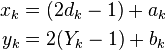
where  and
and  are independent noise components having the same variance
  .
.  is a k-th bit from
  encoder output.
Redundant information is demultiplexed and sent through DI to (when  ) and to (when
  ).
).
yields a soft decision; i.e.:
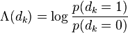
and delivers it to .  is called the logarithm of the likelihood ratio (LLR).
 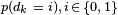 is the a posteriori probability (APP) of the
  data bit which shows the probability of interpreting a received bit as
  . Taking the LLR into account, yields a hard decision; i.e., a decoded bit.
It is known that the Viterbi algorithm is unable to calculate APP, thus it cannot be used in . Instead of that, a modified BCJR algorithm is used. For , the Viterbi algorithm is an appropriate one.
However, the depicted structure is not an optimal one, because uses only a proper fraction of the available redundant information. In order to improve the structure, a feedback loop is used (see the dotted line on the figure).
Soft decision approach
The decoder front-end produces an integer for each bit in the data stream. This integer is a measure of how likely it is that the bit is a 0 or 1 and is also called soft bit. The integer could be drawn from the range [−127, 127], where:
- −127 means "certainly 0"
- −100 means "very likely 0"
- 0 means "it could be either 0 or 1"
- 100 means "very likely 1"
- 127 means "certainly 1"
- etc.
This introduces a probabilistic aspect to the data-stream from the front end, but it conveys more information about each bit than just 0 or 1.
For example, for each bit, the front end of a traditional wireless-receiver has to decide if an internal analog voltage is above or below a given threshold voltage level. For a turbo-code decoder, the front end would provide an integer measure of how far the internal voltage is from the given threshold.
To decode the m + n-bit block of data, the decoder front-end creates a block of likelihood measures, with one likelihood measure for each bit in the data stream. There are two parallel decoders, one for each of the n⁄2-bit parity sub-blocks. Both decoders use the sub-block of m likelihoods for the payload data. The decoder working on the second parity sub-block knows the permutation that the coder used for this sub-block.
Solving hypotheses to find bits
The key innovation of turbo codes is how they use the likelihood data to reconcile differences between the two decoders. Each of the two convolutional decoders generates a hypothesis (with derived likelihoods) for the pattern of m bits in the payload sub-block. The hypothesis bit-patterns are compared, and if they differ, the decoders exchange the derived likelihoods they have for each bit in the hypotheses. Each decoder incorporates the derived likelihood estimates from the other decoder to generate a new hypothesis for the bits in the payload. Then they compare these new hypotheses. This iterative process continues until the two decoders come up with the same hypothesis for the m-bit pattern of the payload, typically in 15 to 18 cycles.
An analogy can be drawn between this process and that of solving cross-reference puzzles like crossword or sudoku. Consider a partially completed, possibly garbled crossword puzzle. Two puzzle solvers (decoders) are trying to solve it: one possessing only the "down" clues (parity bits), and the other possessing only the "across" clues. To start, both solvers guess the answers (hypotheses) to their own clues, noting down how confident they are in each letter (payload bit). Then, they compare notes, by exchanging answers and confidence ratings with each other, noticing where and how they differ. Based on this new knowledge, they both come up with updated answers and confidence ratings, repeating the whole process until they converge to the same solution.
Performance
Turbo codes perform well due to the attractive combination of the code's random appearance on the channel together with the physically realisable decoding structure. Turbo codes are affected by an error floor.
Practical applications using turbo codes
Telecommunications:
- Turbo codes are used extensively in 3G and 4G mobile telephony standards; e.g., in HSPA, EV-DO and LTE.
- MediaFLO, terrestrial mobile television system from Qualcomm.
- The interaction channel of satellite communication systems, such as DVB-RCS.[3]
- New NASA missions such as Mars Reconnaissance Orbiter now use turbo codes, as an alternative to RS-Viterbi codes.
- Turbo coding such as block turbo coding and convolutional turbo coding are used in IEEE 802.16 (WiMAX), a wireless metropolitan network standard.
Bayesian formulation
From an artificial intelligence viewpoint, turbo codes can be considered as an instance of loopy belief propagation in Bayesian networks.[4]
See also
- Convolutional code
- Viterbi algorithm
- Soft-decision decoding
- Interleaver
- BCJR algorithm
- Low-density parity-check code
- Turbo equalizer
References
- ↑ Berrou, Claude; Glavieux, Alain; Thitimajshima, Punya, Near Shannon Limit Error – Correcting, retrieved 11 February 2010
- ↑ Berrou, Claude, The ten-year-old turbo codes are entering into service, Bretagne, France, retrieved 11 February 2010
- ↑ Digital Video Broadcasting (DVB); Interaction channel for Satellite Distribution Systems, ETSI EN 301 790, V1.5.1, May 2009.
- ↑ McEliece, Robert J.; [[David McKay{{subst:DATE}} |MacKay, David J. C.]]; Cheng, Jung-Fu (1998), "Turbo decoding as an instance of Pearl's “belief propagation” algorithm", IEEE Journal on Selected Areas in Communications 16 (2): 140–152, doi:10.1109/49.661103, ISSN 0733-8716.
External links
- "Closing In On The Perfect Code", IEEE Spectrum, March 2004
- "The UMTS Turbo Code and an Efficient Decoder Implementation Suitable for Software-Defined Radios" (International Journal of Wireless Information Networks)
- Dana Mackenzie (2005), "Take it to the limit", New Scientist 187 (2507): 38–41, ISSN 0262-4079. (preview, copy)
- "Pushing the Limit", a Science News feature about the development and genesis of turbo codes
- International Symposium On Turbo Codes
- Coded Modulation Library, an open source library for simulating turbo codes in matlab
- "Turbo Equalization: Principles and New Results", an IEEE Transactions on Communications article about using convolutional codes jointly with channel equalization.
- "PDF Slideshow illustrating the decoding process" A PDF Slideshow illustrating the decoding process
- IT++ Home Page The IT++ is a powerful C++ library which in particular supports turbo codes
- Turbo codes publications by David MacKay
- Extended CML Code including extensive Powerpoint Presentation on Turbo Codes
| ||||||||||||||||||||||||||