Smith–Waterman algorithm
The Smith–Waterman algorithm performs local sequence alignment; that is, for determining similar regions between two strings or nucleotide or protein sequences. Instead of looking at the total sequence, the Smith–Waterman algorithm compares segments of all possible lengths and optimizes the similarity measure.
The algorithm was first proposed by Temple F. Smith and Michael S. Waterman in 1981.[1] Like the Needleman–Wunsch algorithm, of which it is a variation, Smith–Waterman is a dynamic programming algorithm. As such, it has the desirable property that it is guaranteed to find the optimal local alignment with respect to the scoring system being used (which includes the substitution matrix and the gap-scoring scheme). The main difference to the Needleman–Wunsch algorithm is that negative scoring matrix cells are set to zero, which renders the (thus positively scoring) local alignments visible. Backtracking starts at the highest scoring matrix cell and proceeds until a cell with score zero is encountered, yielding the highest scoring local alignment. One does not actually implement the algorithm as described because improved alternatives are now available that have better scaling (Gotoh, 1982) [2] and are more accurate (Altschul and Erickson, 1986).[3]
Explanation
A matrix  is built as follows:


 then
then

 then
then


Where:
-
 = Strings over the Alphabet
-

-

-
 – is the maximum Similarity-Score between a suffix of a[1...i] and a suffix of b[1...j]
 -
 , '–' is the gap-scoring scheme
Example
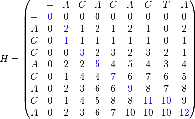
- Sequence 1 = ACACACTA
- Sequence 2 = AGCACACA
|
|
|
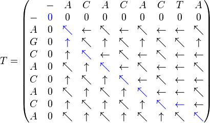
To obtain the optimum local alignment, start with the highest value in the matrix (i,j). Then, go backwards to one of positions (i − 1,j), (i, j − 1), and (i − 1, j − 1) depending on the direction of movement used to construct the matrix. This methodology is maintained until a matrix cell with zero value is reached.
In the example, the highest value corresponds to the cell in position (8,8). The walk back corresponds to (8,8), (7,7), (7,6), (6,5), (5,4), (4,3), (3,2), (2,1), (1,1), and (0,0),
Once finished, the alignment is reconstructed as follows: Starting with the last value, reach (i,j) using the previously calculated path. A diagonal jump implies there is an alignment (either a match or a mismatch). A top-down jump implies there is a deletion. A left-right jump implies there is an insertion.
For the example, the results are:
Sequence 1 = A-CACACTA
Sequence 2 = AGCACAC-A
Motivation
One motivation for local alignment is the difficulty of obtaining correct alignments in regions of low similarity between distantly related biological sequences, because mutations have added too much 'noise' over evolutionary time to allow for a meaningful comparison of those regions. Local alignment avoids such regions altogether and focuses on those with a positive score, i.e. those with an evolutionary conserved signal of similarity. A prerequisite for local alignment is a negative expectation score. The expectation score is defined as the average score that the scoring system (substitution matrix and gap penalties) would yield for a random sequence.
Another motivation for using local alignments is that there is a reliable statistical model (developed by Karlin and Altschul) for optimal local alignments. The alignment of unrelated sequences tends to produce optimal local alignment scores which follow an extreme value distribution. This property allows programs to produce an expectation value for the optimal local alignment of two sequences, which is a measure of how often two unrelated sequences would produce an optimal local alignment whose score is greater than or equal to the observed score. Very low expectation values indicate that the two sequences in question might be homologous, meaning they might share a common ancestor.
The Smith–Waterman algorithm is fairly demanding of time: To align two sequences of lengths m and n, O(mn) time is required. Smith–Waterman local similarity scores can be calculated in O(m) (linear) space if only the optimal alignment needs to be found, but naive algorithms to produce the alignment require O(mn) space. A linear space strategy to find the best local alignment has been described.[4] BLAST and FASTA reduce the amount of time required by identifying conserved regions using rapid lookup strategies, at the cost of exactness.
An implementation of the Smith–Waterman Algorithm, SSEARCH, is available in the FASTA sequence analysis package from . This implementation includes Altivec accelerated code for PowerPC G4 and G5 processors that speeds up comparisons 10–20-fold, using a modification of the Wozniak, 1997 approach,[5] and an SSE2 vectorization developed by Farrar[6] making optimal protein sequence database searches quite practical.
Accelerated versions
FPGA
Cray demonstrated acceleration of the Smith–Waterman algorithm using a reconfigurable computing platform based on FPGA chips, with results showing up to 28x speed-up over standard microprocessor-based solutions. Another FPGA-based version of the Smith–Waterman algorithm shows FPGA (Virtex-4) speedups up to 100x[7] over a 2.2 GHz Opteron processor.[8] The TimeLogic DeCypher and CodeQuest systems also accelerate Smith–Waterman and Framesearch using PCIe FPGA cards.
A 2011 Master's thesis[9] includes an analysis of FPGA-based Smith–Waterman acceleration.
GPU
Lawrence Livermore National Laboratory and the US Department of Energy's Joint Genome Institute implemented an accelerated version of Smith–Waterman local sequence alignment searches using graphics processing units (GPUs) with preliminary results showing a 2x speed-up over software implementations.[10] A similar method has already been implemented in the Biofacet software since 1997, with the same speed-up factor.[11]
Several GPU implementations of the algorithm in NVIDIA's CUDA C platform are also available.[12] When compared to the best known CPU implementation (using SIMD instructions on the x86 architecture), by Farrar, the performance tests of this solution using a single NVidia GeForce 8800 GTX card show a slight increase in performance for smaller sequences, but a slight decrease in performance for larger ones. However the same tests running on dual NVidia GeForce 8800 GTX cards are almost twice as fast as the Farrar implementation for all sequence sizes tested.
A newer GPU CUDA implementation of SW is now available that is faster than previous versions and also removes limitations on query lengths. See CUDASW++.
Eleven different SW implementations on CUDA have been reported, three of which report speedups of 30X.[13]
SIMD
In 2000, a fast implementation of the Smith–Waterman algorithm using the SIMD technology available in Intel Pentium MMX processors and similar technology was described in a publication by Rognes and Seeberg.[14] In contrast to the Wozniak (1997) approach, the new implementation was based on vectors parallel with the query sequence, not diagonal vectors. The company Sencel Bioinformatics has applied for a patent covering this approach. Sencel is developing the software further and provides executables for academic use free of charge.
A SSE2 vectorization of the algorithm (Farrar, 2007) is now available providing an 8-16-fold speedup on Intel/AMD processors with SSE2 extensions.[6] When running on Intel processor using the Core microarchitecture the SSE2 implementation achieves a 20-fold increase. Farrar's SSE2 implementation is available as the SSEARCH program in the FASTA sequence comparison package. The SSEARCH is included in the European Bioinformatics Institute's suite of similarity searching programs.
Danish bioinformatics company CLC bio has achieved speed-ups of close to 200 over standard software implementations with SSE2 on an Intel 2.17 GHz Core 2 Duo CPU, according to a publicly available white paper.
Accelerated version of the Smith–Waterman algorithm, on Intel and AMD based Linux servers, is supported by the GenCore 6 package, offered by Biocceleration. Performance benchmarks of this software package show up to 10 fold speed acceleration relative to standard software implementation on the same processor.
Currently the only company in bioinformatics to offer both SSE and FPGA solutions accelerating Smith–Waterman, CLC bio has achieved speed-ups of more than 110 over standard software implementations with CLC Bioinformatics Cube [citation needed]
The fastest implementation of the algorithm on CPUs with SSSE3 can be found the SWIPE software (Rognes, 2011),[15] which is available under the GNU Affero General Public License. In parallel, this software compares residues from sixteen different database sequences to one query residue. Using a 375 residue query sequence a speed of 106 billion cell updates per second (GCUPS) was achieved on a dual Intel Xeon X5650 six-core processor system, which is over six times more rapid than software based on Farrar's 'striped' approach. It is faster than BLAST when using the BLOSUM50 matrix.
Cell Broadband Engine
In 2008, Farrar[16] described a port of the Striped Smith–Waterman[6] to the Cell Broadband Engine and reported speeds of 32 and 12 GCUPS on an IBM QS20 blade and a Sony PlayStation 3, respectively.
See also
- BLAST
- Sequence mining
- FASTA
- Levenshtein distance
- Needleman–Wunsch algorithm
References
- ↑ Smith, Temple F.; and Waterman, Michael S. (1981). "Identification of Common Molecular Subsequences". Journal of Molecular Biology 147: 195–197. doi:10.1016/0022-2836(81)90087-5. PMID 7265238.
- ↑ Osamu Gotoh (1982). "An improved algorithm for matching biological sequences". Journal of molecular biology 162: 705.
- ↑ Stephen F. Altschul; and Bruce W. Erickson (1986). "Optimal sequence alignment using affine gap costs". Bulletin of Mathematical Biology 48: 603–616. doi:10.1007/BF02462326.
- ↑ Miller, Webb and Myers, Eugene (1988). "Optimal alignments in linear space". Computer Applications in Biosciences (CABIOS) 4: 11–17.
- ↑ Wozniak, Andrzej (1997). "Using video-oriented instructions to speed up sequence comparison". Computer Applications in Biosciences (CABIOS) 13 (2): 145–50.
- ↑ 6.0 6.1 6.2 Farrar, Michael S. (2007). "Striped Smith–Waterman speeds database searches six times over other SIMD implementations". Bioinformatics 23 (2): 156–161. doi:10.1093/bioinformatics/btl582. PMID 17110365.
- ↑ FPGA 100x Papers: , , and
- ↑ Progeniq Pte. Ltd., "White Paper - Accelerating Intensive Applications at 10×–50× Speedup to Remove Bottlenecks in Computational Workflows".
- ↑ Genetic sequence alignment on a supercomputing platform ""
- ↑ "GPU Accelerated Smith–Waterman". SpringerLink.
- ↑ "Bioinformatics High Throughput Sequence Search and Analysis (white paper)". GenomeQuest. Retrieved 2008-05-09.
- ↑ "CUDA Zone". Nvidia. Retrieved 2010-02-25.
- ↑ Rognes, Torbjørn; and Seeberg, Erling (2000). "Six-fold speed-up of Smith–Waterman sequence database searches using parallel processing on common microprocessors". Bioinformatics 16 (8): 699–706.
- ↑ Rognes, Torbjørn (2011). "Faster Smith–Waterman database searches with inter-sequence SIMD parallelisation". BMC Bioinformatics 12: 221. doi:10.1186/1471-2105-12-221. PMC 3120707. PMID 21631914.
- ↑ Farrar, Michael S. (2008). Optimizing Smith–Waterman for the Cell Broadband Engine.
External links
- JAligner — an open source Java implementation of the Smith–Waterman algorithm
- B.A.B.A. — an applet (with source) which visually explains the algorithm.
- FASTA/SSEARCH at the EBI's FASTA/SSEARCH services page.
- UGENE Smith–Waterman plugin — An open source SSEARCH compatible implementation of the algorithm with graphical interface written in C++.
- OPAL JavaScript implementation of algorithms: Needleman–Wunsch, Needleman–Wunsch–Sellers and Smith–Waterman


