Radon transform

From Wikipedia, the free encyclopedia

Radon transform.

Radon transform of the indicator function of two squares shown in the image below. Lighter regions indicate larger function values. Black indicates zero.

Original function is equal to one on the white region and zero on the dark region.

In mathematics, the Radon transform in two dimensions, named after the Austrian mathematician Johann Radon, is the integral transform consisting of the integral of a function over straight lines. The transform was introduced by Johann Radon (1917), who also provided a formula for the inverse transform. Radon further included formulas for the transform in three-dimensions, in which the integral is taken over planes. It was later generalised to higher-dimensional Euclidean spaces, and more broadly in the context of integral geometry. The complex analog of the Radon transform is known as the Penrose transform.

Shepp Logan phantom

Radon transform

Inverse Radon transform

The Radon transform is widely applicable to tomography, the creation of an image from the scattering data associated with cross-sectional scans of an object. If a function ƒ represents an unknown density, then the Radon transform represents the scattering data obtained as the output of a tomographic scan. Hence the inverse of the Radon transform can be used to reconstruct the original density from the scattering data, and thus it forms the mathematical underpinning for tomographic reconstruction, also known as image reconstruction. The Radon transform data is often called a sinogram because the Radon transform of a Dirac delta function is a distribution supported on the graph of a sine wave. Consequently the Radon transform of a number of small objects appears graphically as a number of blurred sine waves with different amplitudes and phases. The Radon transform is useful in computed axial tomography (CAT scan), barcode scanners, electron microscopy of macromolecular assemblies like viruses and protein complexes, reflection seismology and in the solution of hyperbolic partial differential equations.

Definition

Let ƒ(x) = ƒ(x,y) be a continuous function vanishing outside some large disc in the Euclidean plane R². The Radon transform, Rƒ, is a function defined on the space of straight lines L in R² by the line integral along each such line:

$Rf(L)=\int _{L}f({\mathbf {x}})\,|d{\mathbf {x}}|.$

Concretely, the parametrization of any straight line L with respect to arc length t can always be written

$(x(t),y(t))={\Big (}(t\sin \alpha +s\cos \alpha ),(-t\cos \alpha +s\sin \alpha ){\Big )}\,$

where s is the distance of L from the origin and $\alpha$ is the angle the normal vector to L makes with the x axis. It follows that the quantities (α,s) can be considered as coordinates on the space of all lines in R², and the Radon transform can be expressed in these coordinates by

${\begin{aligned}Rf(\alpha ,s)&=\int _{{-\infty }}^{{\infty }}f(x(t),y(t))\,dt\\&=\int _{{-\infty }}^{{\infty }}f{\big (}(t\sin \alpha +s\cos \alpha ),(-t\cos \alpha +s\sin \alpha ){\big )}\,dt\end{aligned}}$

More generally, in the n-dimensional Euclidean space Rⁿ, the Radon transform of a compactly supported continuous function ƒ is a function Rƒ on the space Σ_n of all hyperplanes in Rⁿ. It is defined by

$Rf(\xi )=\int _{\xi }f({\mathbf {x}})\,d\sigma ({\mathbf {x}})$

for ξ ∈Σ_n, where the integral is taken with respect to the natural hypersurface measure, dσ (generalizing the |dx| term from the 2-dimensional case). Observe that any element of Σ_n is characterized as the solution locus of an equation

${\mathbf {x}}\cdot \alpha =s$

where α ∈ Sⁿ⁻¹ is a unit vector and s ∈ R. Thus the n-dimensional Radon transform may be rewritten as a function on Sⁿ⁻¹×R via

$Rf(\alpha ,s)=\int _{{{\mathbf {x}}\cdot \alpha =s}}f({\mathbf {x}})\,d\sigma ({\mathbf {x}}).$

It is also possible to generalize the Radon transform still further by integrating instead over k-dimensional affine subspaces of Rⁿ. The X-ray transform is the most widely used special case of this construction, and is obtained by integrating over straight lines.

Relationship with the Fourier transform

Main article: Projection-slice theorem

The Radon transform is closely related to the Fourier transform. For a function of one variable the Fourier transform is defined by

${\hat {f}}(\omega )=\int _{{-\infty }}^{\infty }f(x)e^{{-2\pi ix\omega }}\,dx.$

and for a function of a 2-vector ${\mathbf {x}}=(x,y)$ ,

${\hat {f}}({\mathbf {w}})=\int \limits _{{-\infty }}^{{\infty }}\int \limits _{{-\infty }}^{{\infty }}f({\mathbf {x}})e^{{-2\pi i{\mathbf {x}}\cdot {\mathbf {w}}}}\,dx\,dy.$

For convenience define $R_{\alpha }[f](s)=R[f](\alpha ,s)$ as it is only meaningful to take the Fourier transform in the $s$ variable. The Fourier slice theorem then states

$\widehat {R_{{\alpha }}[f]}(\sigma )={\hat {f}}(\sigma {\mathbf {n}}(\alpha ))$

where

${\mathbf {n}}(\alpha )=(\cos \alpha ,\sin \alpha ).$

Thus the two-dimensional Fourier transform of the initial function is the one variable Fourier transform of the Radon transform of that function. More generally, one has the result valid in n dimensions

${\hat {f}}(r\alpha )=\int _{{-\infty }}^{\infty }Rf(\alpha ,s)e^{{-2\pi isr}}\,ds.$

Indeed, the result follows at once by computing the two variable Fourier integral along appropriate slices:

${\hat {f}}(r\alpha )=\int _{{-\infty }}^{\infty }ds\int _{{{\mathbf {x}}\cdot \alpha =s}}e^{{-2\pi ir({\mathbf {x}}\cdot \alpha )}}dm({\mathbf {x}}).$

An application of the Fourier inversion formula also gives an explicit inversion formula for the Radon transform, and thus shows that it is invertible on suitably chosen spaces of functions. However this form is not particularly useful for numerical inversion, and faster discrete inversion methods exist.

Dual transform

The dual Radon transform is a kind of adjoint to the Radon transform. Beginning with a function g on the space Σ_n, the dual Radon transform is the function R^∗g on Rⁿ defined by

$R^{*}g(x)=\int _{{x\in \xi }}g(\xi )\,d\mu (\xi ).$

The integral here is taken over the set of all lines incident with the point x ∈ Rⁿ, and the measure dμ is the unique probability measure on the set $\{\xi |x\in \xi \}$ invariant under rotations about the point x.

Concretely, for the two-dimensional Radon transform, the dual transform is given by

$R^{*}g(x)={\frac {1}{2\pi }}\int _{{\alpha =0}}^{{2\pi }}g(\alpha ,{\mathbf {n}}(\alpha )\cdot {\mathbf {x}})\,d\alpha .$

In the context of image processing, the dual transform is commonly called backprojection^[1] as it takes a function defined on each line in the plane and 'smears' or projects it back over the line to produce an image. Computationally efficient inversion formulas reconstruct the image from the points where the back-projection lines meet.

Intertwining property

Let Δ denote the Laplacian on Rⁿ:

$\Delta ={\frac {\partial ^{2}}{\partial x_{1}^{2}}}+\cdots +{\frac {\partial ^{2}}{\partial x_{n}^{2}}}.$

This is a natural rotationally invariant second-order differential operator. On Σ_n, the "radial" second derivative

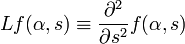
$Lf(\alpha ,s)\equiv {\frac {\partial ^{2}}{\partial s^{2}}}f(\alpha ,s)$

is also rotationally invariant. The Radon transform and its dual are intertwining operators for these two differential operators in the sense that^[2]

$R(\Delta f)=L(Rf),\quad R^{*}(Lg)=\Delta (R^{*}g).$

Inversion formulas

Explicit and computationally efficient inversion formulas for the Radon transform and its dual are available. The Radon transform in n dimensions can be inverted by the formula^[3]

$c_{n}f=(-\Delta )^{{(n-1)/2}}R^{*}Rf\,$

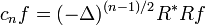
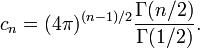
where

$c_{n}=(4\pi )^{{(n-1)/2}}{\frac {\Gamma (n/2)}{\Gamma (1/2)}}.$

and the power of the Laplacian (−Δ)^(n−1)/2 is defined as a pseudodifferential operator if necessary by the Fourier transform

${\mathcal {F}}\left[(-\Delta )^{{(n-1)/2}}\phi \right](\xi )=|2\pi \xi |^{{n-1}}{\mathcal {F}}\phi (\xi ).$

For computational purposes, the power of the Laplacian is commuted with the dual transform R^* to give^[4]

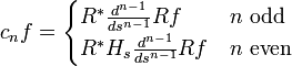
$c_{n}f={\begin{cases}R^{*}{\frac {d^{{n-1}}}{ds^{{n-1}}}}Rf&n{\rm {{\ odd}}}\\R^{*}H_{s}{\frac {d^{{n-1}}}{ds^{{n-1}}}}Rf&n{\rm {{\ even}}}\end{cases}}$

where H_s is the Hilbert transform with respect to the s variable. In two dimensions, the operator H_sd/ds appears in image processing as a ramp filter.^[5] One can prove directly from the Fourier slice theorem and change of variables for integration that for a compactly supported continuous function ƒ of two variables

$f={\frac {1}{2}}R^{{*}}H_{s}{\frac {d}{ds}}Rf.$

Thus in an image processing context the original image ƒ can be recovered from the 'sinogram' data Rƒ by applying a ramp filter (in the $s$ variable) and then back-projecting. As the filtering step can be performed efficiently (for example using digital signal processing techniques) and the back projection step is simply an accumulation of values in the pixels of the image, this results in a highly efficient, and hence widely used, algorithm.

Explicitly, the inversion formula obtained by the latter method is^[1]

$f(x)={\frac {1}{2}}(2\pi )^{{1-n}}(-1)^{{(n-1)/2}}\int _{{S^{{n-1}}}}{\frac {\partial ^{{n-1}}}{\partial s^{{n-1}}}}Rf(\alpha ,\alpha \cdot x)\,d\alpha$

if n is odd, and

$f(x)=(2\pi )^{{-n}}(-1)^{{n/2}}\int _{{-\infty }}^{\infty }{\frac {1}{q}}\int _{{S^{{n-1}}}}{\frac {\partial ^{{n-1}}}{\partial s^{{n-1}}}}Rf(\alpha ,\alpha \cdot x+q)\,d\alpha \,dq$

if n is even.

The dual transform can also be inverted by an analogous formula:

$c_{n}g=(-L)^{{(n-1)/2}}R(R^{*}g).\,$

Notes

↑ 1.0 1.1 Roerdink 2001
↑ Helgason 1984, Lemma I.2.1
↑ Helgason 1984, Theorem I.2.13
↑ Helgason 1984, Theorem I.2.16
↑ Filtered Back Projection
↑ http://www.tnw.tudelft.nl/live/pagina.jsp?id=45028650-24bd-4b30-9ada-b11aaca457c0&lang=en&binary=/doc/mvanginkel_radonandhough_tr2004.pdf

References

Deans, Stanley R. (1983), The Radon Transform and Some of Its Applications, New York: John Wiley & Sons .
Helgason, Sigurdur (2008), Geometric analysis on symmetric spaces, Mathematical Surveys and Monographs 39 (2nd ed.), Providence, R.I.: American Mathematical Society, ISBN 978-0-8218-4530-1, MR 2463854 .
Helgason, Sigurdur (1984), Groups and Geometric Analysis: Integral Geometry, Invariant Differential Operators, and Spherical Functions, Academic Press, ISBN 0-12-338301-3 .
Herman, Gabor T. (2009), Fundamentals of Computerized Tomography: Image Reconstruction from Projections (2nd ed.), Springer, ISBN 978-1-85233-617-2 .
Minlos, R.A. (2001), "Radon transform", in Hazewinkel, Michiel, Encyclopedia of Mathematics, Springer, ISBN 978-1-55608-010-4 .
Natterer, Frank, The Mathematics of Computerized Tomography, Classics in Applied Mathematics 32, Society for Industrial and Applied Mathematics, ISBN 0-89871-493-1
Natterer, Frank; Wübbeling, Frank, Mathematical Methods in Image Reconstruction, Society for Industrial and Applied Mathematics, ISBN 0-89871-472-9 .
Radon, Johann (1917), "Über die Bestimmung von Funktionen durch ihre Integralwerte längs gewisser Mannigfaltigkeiten", Berichte über die Verhandlungen der Königlich-Sächsischen Akademie der Wissenschaften zu Leipzig, Mathematisch-Physische Klasse [Reports on the proceedings of the Royal Saxonian Academy of Sciences at Leipzig, mathematical and physical section] (Leipzig: Teubner) (69): 262–277 ; Translation: Radon, J.; Parks, P.C. (translator) (1986), "On the determination of functions from their integral values along certain manifolds", IEEE Transactions on Medical Imaging 5 (4): 170–176, doi:10.1109/TMI.1986.4307775, PMID 18244009 .
Roerdink, J.B.T.M. (2001), "Tomography", in Hazewinkel, Michiel, Encyclopedia of Mathematics, Springer, ISBN 978-1-55608-010-4 .
Weisstein, Eric W., "Radon transform", MathWorld..

This article is issued from Wikipedia. The text is available under the Creative Commons Attribution/Share Alike; additional terms may apply for the media files.

Radon transform

Definition

Relationship with the Fourier transform

Dual transform

Intertwining property

Inversion formulas

See also

Notes

References