Ponderomotive force
In physics, a ponderomotive force is a nonlinear force that a charged particle experiences in an inhomogeneous oscillating electromagnetic field.
The ponderomotive force Fp is expressed by


where e is the electrical charge of the particle, m is the mass, ω is the angular frequency of oscillation of the field, and E is the amplitude of the electric field (at low enough amplitudes the magnetic field exerts very little force).
This equation means that a charged particle in an inhomogeneous oscillating field not only oscillates at the frequency of ω but also drifts toward the weak field area. It is noteworthy that this is one rare case where the sign of the particle charge does not change the direction of the force, unlike the Lorentz force.
The mechanism of the ponderomotive force can be easily understood by considering the motion of the charge in an oscillating electric field. In the case of a homogeneous field, the charge returns to its initial position after one cycle of oscillation. In the case of an inhomogeneous field, the force exerted on the charge during the half-cycle it spends in the area with higher field amplitude points towards the weak field area. It is larger than the force exerted during the half-cycle spent in the area with a lower field amplitude, which points towards the strong field area. Thus, averaged over a full cycle there is a net force that drives the charge toward the weak field area.
Derivation
The derivation of the ponderomotive force expression proceeds as follows.
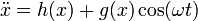
Consider a particle under the action of a non-uniform oscillating field. The equation of motion is given by:

neglecting the effect of the associated oscillating magnetic field.
If the length scale of variation of  is large enough, then the particle trajectory can be divided into a slow time motion and a fast time motion:[1]

where  is the slow drift motion and
  represents fast oscillations. Now, let us also assume that
  . Under this assumption, we can use Taylor expansion on the force equation about to get,
![{\ddot {x_{0}}}+{\ddot {x_{1}}}=\left[g(x_{0})+x_{1}g'(x_{0})\right]\cos(\omega t)](/2014-wikipedia_en_all_02_2014/I/media/a/7/1/9/a719fc8eae1b131358932975f806e3d0.png)
 , and because is small,
  , so
, so
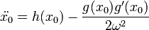
On the time scale on which oscillates, is essentially a constant. Thus, the above can be integrated to get,
Substituting this in the force equation and averaging over the  timescale, we get,
![\Rightarrow {\ddot {x_{0}}}=-{\frac {1}{4\omega ^{2}}}\left.{\frac {d}{dx}}\left[g(x)^{2}\right]\right|_{{x=x_{0}}}](/2014-wikipedia_en_all_02_2014/I/media/d/2/d/c/d2dca8678f4b20ca6195ec34eef89c26.png)
Thus, we have obtained an expression for the drift motion of a charged particle under the effect of a non-uniform oscillating field.
Time averaged Density
Instead of a single charged particle, there could be a gas of charged particles confined by the action of such a force. Such a gas of charged particles is called plasma. The distribution function and density of the plasma will fluctuate at the applied oscillating frequency and to obtain an exact solution, we need to solve the Vlasov Equation. But, it is usually assumed that the time averaged density of the plasma can be directly obtained from the expression for the force expression for the drift motion of individual charged particles:[2]
![{\bar {n}}(x)=n_{0}\exp \left[-{\frac {e}{\kappa T}}\Phi _{{{\text{P}}}}(x)\right]](/2014-wikipedia_en_all_02_2014/I/media/a/f/6/1/af61154a875a37fa403872c19f72d798.png)
where  is the ponderomotive potential and is given by
![\Phi _{{{\text{P}}}}(x)={\frac {m}{4\omega ^{2}}}\left[g(x)\right]^{2}](/2014-wikipedia_en_all_02_2014/I/media/5/b/4/9/5b495bb0cfbfb490a39b0ce9d866f6af.png)
Generalized Ponderomotive Force
Instead of just an oscillating field, there could also be a permanent field present. In such a situation, the force equation of a charged particle becomes:
To solve the above equation, we can make a similar assumption as we did for the case when  . This gives a generalized expression for the drift motion of the particle:
Applications
The idea of a ponderomotive description of particles under the action of a time varying field has applications in areas like:
- Quadrupole ion trap
- Combined rf trap
- Plasma acceleration of particles
- Plasma propulsion engine especially the Electrodeless plasma thruster
- High Harmonic Generation
- Terahertz time-domain spectroscopy as a source of high energy THz radiation in laser-induced air plasmas
The ponderomotive force also plays an important role in laser induced plasmas as a major density lowering factor.
References
- General
- Schmidt, George (1979). Physics of High Temperature Plasmas, second edition. Academic Press. p. 47. ISBN 0-12-626660-3.
- Citations
- ↑ Introduction to Plasma Theory, second edition, by Nicholson, Dwight R., Wiley Publications (1983), ISBN 0-471-09045-X
- ↑ V. B. Krapchev, Kinetic Theory of the Ponderomotive Effects in a Plasma, Phys. Rev. Lett. 42, 497 (1979), http://prola.aps.org/abstract/PRL/v42/i8/p497_1
Journals
- J. R. Cary and A. N. Kaufman, Ponderomotive effects in collisionless plasma: A Lie transform approach, Phys. Fluids 24, 1238 (1981), http://dx.doi.org/10.1063/1.863527
- C. Grebogi and R. G. Littlejohn, Relativistic ponderomotive Hamiltonian, Phys. Fluids 27, 1996 (1984), http://dx.doi.org/10.1063/1.864855
- G. J. Morales and Y. C. Lee, Ponderomotive-Force Effects in a Nonuniform Plasma, Phys. Rev. Lett. 33, 1016 (1974), http://prola.aps.org/abstract/PRL/v33/i17/p1016_1
- B. M. Lamb and G. J. Morales, Ponderomotive effects in nonneutral plasmas, Phys. Fluids 26, 3488 (1983), http://dx.doi.org/10.1063/1.864132
- K. Shah and H. Ramachandran, Analytic, nonlinearly exact solutions for an rf confined plasma, Phys. Plasmas 15, 062303 (2008), http://link.aip.org/link/?PHPAEN/15/062303/1
- P. H. Bucksbaum, R. R. Freeman, M. Bashkansky, and T. J. McIlrath, Role of the ponderomotive potential in above-threshold ionization, Jour. Opt. Soc. B 4, 760 (1987), http://www.opticsinfobase.org/josab/abstract.cfm?uri=josab-4-5-760