Planckian locus
In physics and color science, the Planckian locus or black body locus is the path or locus that the color of an incandescent black body would take in a particular chromaticity space as the blackbody temperature changes. It goes from deep red at low temperatures through orange, yellowish white, white, and finally bluish white at very high temperatures.
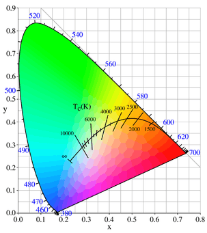
A color space is a three-dimensional space; that is, a color is specified by a set of three numbers (the CIE coordinates X, Y, and Z, for example, or other values such as hue, colorfulness, and luminance) which specify the color and brightness of a particular homogeneous visual stimulus. A chromaticity is a color projected into a two-dimensional space that ignores brightness. For example, the standard CIE XYZ color space projects directly to the corresponding chromaticity space specified by the two chromaticity coordinates known as x and y, making the familiar chromaticity diagram shown in the figure. The Planckian locus, the path that the color of a black body takes as the blackbody temperature changes, is often shown in this standard chromaticity space.
The Planckian locus in the XYZ color space

In the CIE XYZ color space, the three coordinates defining a color are given by X, Y, and Z:[1]


where I(λ,T) is the spectral radiance of the light being viewed, and X(λ), Y(λ) and Z(λ) are the color matching functions of the CIE standard colorimetric observer, shown in the diagram on the right, and λ is the wavelength. The Planckian locus is determined by substituting into the above equations the black body spectral radiance, which is given by Planck's law:

where:
- I is the black body spectral radiance (power per unit area per unit solid angle per unit wavelength)
- T is the temperature of the black body
- h is Planck's constant
- c is the speed of light
- k is Boltzmann's constant
This will give the Planckian locus in CIE XYZ color space. If these coordinates are XT, YT, ZT where T is the temperature, then in the CIE chromaticity coordinates will be


Approximation
The Planckian locus in xy space is depicted as a curve in the chromaticity diagram above. While it is possible to compute the CIE xy co-ordinates exactly given the above formulas, it is faster to use approximations. Since the mired scale changes more evenly along the locus than the temperature itself, it is common for such approximations to be functions of the reciprocal temperature. Kim et al. uses a cubic spline:[2][3]


The inverse calculation, from chromaticity co-ordinates (x,y) on or near the Planckian locus to correlated color temperature, is discussed in Color temperature#Approximation.
The Planckian locus can also be approximated in the CIE 1960 UCS, which is used to compute CCT and CRI, using the following expressions:[4]


This approximation is accurate to within  and
and  for
for 
Correlated color temperature
The correlated color temperature (Tcp) is the temperature of the Planckian radiator whose perceived colour most closely resembles that of a given stimulus at the same brightness and under specified viewing conditions
The mathematical procedure for determining the correlated color temperature involves finding the closest point to the light source's white point on the Planckian locus. Since the CIE's 1959 meeting in Brussels, the Planckian locus has been computed using the CIE 1960 color space, also known as MacAdam's (u,v) diagram.[6] Today, the CIE 1960 color space is deprecated for other purposes:[7]
The 1960 UCS diagram and 1964 Uniform Space are declared obsolete recommendation in CIE 15.2 (1986), but have been retained for the time being for calculating colour rendering indices and correlated colour temperature.
Owing to the perceptual inaccuracy inherent to the concept, it suffices to calculate to within 2K at lower CCTs and 10K at higher CCTs to reach the threshold of imperceptibility.[8]


International Temperature Scale
The Planckian locus is derived by the determining the chromaticity values of a Planckian radiator using the standard colorimetric observer. The relative spectral power distribution (SPD) of a Planckian radiator follows Planck's law, and depends on the second radiation constant,  . As measuring techniques have improved, the General Conference on Weights and Measures has revised its estimate of this constant, with the International Temperature Scale (and briefly, the International Practical Temperature Scale). These successive revisions caused a shift in the Planckian locus and, as a result, the correlated color temperature scale. Before ceasing publication of standard illuminants, the CIE worked around this problem by explicitly specifying the form of the SPD, rather than making references to black bodies and a color temperature. Nevertheless, it is useful to be aware of previous revisions in order to be able to verify calculations made in older texts:[9][10]
-
 (ITS-27). Note: Was in effect during the standardization of Illuminants A, B, C (1931), however the CIE used the value recommended by the U.S. National Bureau of Standards, 1.435 × 10⁻²[11][12]
 -
 (IPTS-48). In effect for Illuminant series D (formalized in 1967).
 -
 (ITS-68), (ITS-90). Often used in recent papers.
 -
 (CODATA, 2006). Current value, as of 2008.[13]
References
- ↑ Wyszecki, Günter and Stiles, Walter Stanley (2000). Color Science: Concepts and Methods, Quantitative Data and Formulae (2E ed.). Wiley-Interscience. ISBN 0-471-39918-3.
- ↑ US patent 7024034, Kim et al., "Color Temperature Conversion System and Method Using the Same", issued 2006-04-04
- ↑ Bongsoon Kang, Ohak Moon, Changhee Hong, Honam Lee, Bonghwan Cho and Youngsun Kim (December 2002). "Design of Advanced Color Temperature Control System for HDTV Applications". Journal of the Korean Physical Society 41 (6): 865–871.
- ↑ Krystek, Michael P. (January 1985). "An algorithm to calculate correlated colour temperature". Color Research & Application 10 (1): 38–40. doi:10.1002/col.5080100109. "A new algorithm to calculate correlated colour temperature is given. This algorithm is based on a rational Chebyshev approximation of the Planckian locus in the CIE 1960 UCS diagram and a bisection procedure. Thus time-consuming search procedures in tables or charts are no longer necessary."
- ↑ Borbély, Ákos; Sámson,Árpád;Schanda, János (December 2001). "The concept of correlated colour temperature revisited". Color Research & Application 26 (6): 450–457. doi:10.1002/col.1065.
- ↑ Kelly, Kenneth L. (August 1963). "Lines of constant correlated color temperature based on MacAdam's (u,v) Uniform chromaticity transformation of the CIE diagram" (abstract). JOSA 53 (8): 999. doi:10.1364/JOSA.53.000999.
- ↑ Simons, Ronald Harvey; Bean, Arthur Robert (2001). Lighting Engineering: Applied Calculations. Architectural Press. ISBN 0-7506-5051-6.
- ↑ Ohno, Yoshi; Jergens, Michael (19 June 1999). "Results of the Intercomparison of Correlated Color Temperature Calculation". CORM.
- ↑ Janos Schanda (2007). "3: CIE Colorimetry". Colorimetry: Understanding the CIE System. Wiley Interscience. pp. 37–46. ISBN 978-0-470-04904-4.
- ↑ The ITS-90 Resource Site
- ↑ Hall, J.A. (January 1967). "The Early History of the International Practical Scale of Temperature". Metrologia 3 (1): 25–28. doi:10.1088/0026-1394/3/1/006.
- ↑ Moon, Parry (March 1948). "A table of Planckian radiation" (abstract). JOSA 38 (3): 291–294. doi:10.1364/JOSA.38.000291.
- ↑ Mohr, Peter J.; Taylor, Barry N. and Newell, David B. (2007). "CODATA Recommended Values of the Fundamental Physical Constants: 2006".
External links
- Numerical table of color temperature and the corresponding xy and sRGB coordinates for both the 1931 and 1964 CMFs, by Mitchell Charity.