Negative temperature

From Wikipedia, the free encyclopedia

SI temperature/coldness (1/kT) scale.

In physics, certain systems can achieve negative temperature; that is, their thermodynamic temperature can be expressed as a negative quantity on the Kelvin or Rankine scales. In colloquial usage, "negative temperature" may refer to temperatures that are expressed as negative numbers on the more familiar Celsius or Fahrenheit scales, with values that are colder than the zero points of those scales but still warmer than absolute zero. By contrast, a system with a truly negative temperature in absolute terms on the Kelvin scale is hotter than any system with a positive temperature. If a negative-temperature system and a positive-temperature system come in contact, heat will flow from the negative- to the positive-temperature system.^[1]^[2]

That a system at negative temperature is hotter than any system at positive temperature is paradoxical if absolute temperature is interpreted as an average kinetic energy of the system. The paradox is resolved by understanding temperature through its more rigorous definition as the tradeoff between energy and entropy, with the reciprocal of the temperature, thermodynamic beta, as the more fundamental quantity. Systems with a positive temperature will increase in entropy as one adds energy to the system. Systems with a negative temperature will decrease in entropy as one adds energy to the system.^[3]

Most familiar systems cannot achieve negative temperatures, because adding energy always increases their entropy. The possibility of decreasing in entropy with increasing energy requires the system to "saturate" in entropy, with the number of high energy states being small. These kinds of systems, bounded by a maximum amount of energy, are generally forbidden classically. Thus, negative temperature is a strictly quantum phenomenon. Some systems, however (see the examples below), have a maximum amount of energy that they can hold, and as they approach that maximum energy their entropy actually begins to decrease.^[4]

Heat and molecular energy distribution

Negative temperatures can only exist in a system where there are a limited number of energy states (see below). As the temperature is increased on such a system, particles move into higher and higher energy states, and as the temperature increases, the number of particles in the lower energy states and in the higher energy states approaches equality. (This is a consequence of the definition of temperature in statistical mechanics for systems with limited states.) By injecting energy into these systems in the right fashion, it is possible to create a system in which there are more particles in the higher energy states than in the lower ones. The system can then be characterised as having a negative temperature. A substance with a negative temperature is not colder than absolute zero, but rather it is hotter than infinite temperature. As Kittel and Kroemer (p. 462) put it, "The temperature scale from cold to hot runs:

+0 K, ... , +300 K, ... , +∞ K, −∞ K, ... , −300 K, ... , −0 K."

Generally, temperature as it is felt is defined by the kinetic energy of atoms. Since there is no upper bound on momentum of an atom there is no upper bound to the number of energy states available if enough energy is added, and no way to get to a negative temperature. However, temperature is more generally defined by statistical mechanics than just kinetic energy (see below). The inverse temperature β = 1/kT (where k is Boltzmann's constant) scale runs continuously from low energy to high as +∞, ... , −∞.

Temperature and disorder

The distribution of energy among the various translational, vibrational, rotational, electronic, and nuclear modes of a system determines the macroscopic temperature. In a "normal" system, thermal energy is constantly being exchanged between the various modes.

However, for some cases, it is possible to isolate one or more of the modes. In practice, the isolated modes still exchange energy with the other modes, but the time scale of this exchange is much slower than for the exchanges within the isolated mode. One example is the case of nuclear spins in a strong external magnetic field. In this case, energy flows fairly rapidly among the spin states of interacting atoms, but energy transfer between the nuclear spins and other modes is relatively slow. Since the energy flow is predominantly within the spin system, it makes sense to think of a spin temperature that is distinct from the temperature due to other modes.

A definition of temperature can be based on the relationship:

$T={\frac {dq_{{\mathrm {rev}}}}{dS}}$

The relationship suggests that a positive temperature corresponds to the condition where entropy, S, increases as thermal energy, q_rev, is added to the system. This is the "normal" condition in the macroscopic world, and is always the case for the translational, vibrational, rotational, and non-spin related electronic and nuclear modes. The reason for this is that there are an infinite number of these types of modes, and adding more heat to the system increases the number of modes that are energetically accessible, and thus increases the entropy.

Examples

Noninteracting two–level particles

Entropy, thermodynamic beta, and temperature as a function of the energy for a system of N noninteracting two–level particles.

The simplest example, albeit a rather nonphysical one, is to consider a system of N particles, each of which can take an energy of either +ε or -ε but are otherwise noninteracting. This can be understood as a limit of the Ising model in which the interaction term becomes negligible. The total energy of the system is

$E=\epsilon \sum _{{i=1}}^{N}\sigma _{i}=\epsilon \cdot j$

where σ_i is the sign of the ith particle and j is the number of particles with positive energy minus the number of particles with negative energy. From elementary combinatorics, the total number of microstates with this amount of energy is a binomial coefficient:

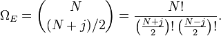
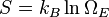
$\Omega _{E}={\binom {N}{(N+j)/2}}={\frac {N!}{\left({\frac {N+j}{2}}\right)!\left({\frac {N-j}{2}}\right)!}}.$

By the fundamental assumption of statistical mechanics, the entropy of this microcanonical ensemble is

$S=k_{B}\ln \Omega _{E}$

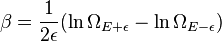
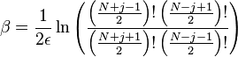
We can solve for thermodynamic beta (β = 1/k_BT) by considering it as a central difference without taking the continuum limit:

$\beta ={\frac {1}{k_{B}}}{\frac {\delta _{{2\epsilon }}[S]}{2\epsilon }}$

$\beta ={\frac {1}{2\epsilon }}(\ln \Omega _{{E+\epsilon }}-\ln \Omega _{{E-\epsilon }})$

$\beta ={\frac {1}{2\epsilon }}\ln \left({\frac {\left({\frac {N+j-1}{2}}\right)!\left({\frac {N-j+1}{2}}\right)!}{\left({\frac {N+j+1}{2}}\right)!\left({\frac {N-j-1}{2}}\right)!}}\right)$

$\beta ={\frac {1}{2\epsilon }}\ln \left({\frac {N-j+1}{N+j+1}}\right).$

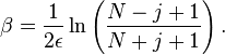
hence the temperature

$T(E)={\frac {2\epsilon }{k_{B}}}\left[\ln \left({\frac {(N+1)\epsilon -E}{(N+1)\epsilon +E}}\right)\right]^{{-1}}.$

Nuclear spins

The previous example is an approximate realization of a system of nuclear spins in an external magnetic field.^[5]^[6] In the case of electronic and nuclear spin systems, there are only a finite number of modes available, often just two, corresponding to spin up and spin down. In the absence of a magnetic field, these spin states are degenerate, meaning that they correspond to the same energy. When an external magnetic field is applied, the energy levels are split, since those spin states that are aligned with the magnetic field will have a different energy from those that are anti-parallel to it.

In the absence of a magnetic field, such a two-spin system would have maximum entropy when half the atoms are in the spin-up state and half are in the spin-down state, and so one would expect to find the system with close to an equal distribution of spins. Upon application of a magnetic field, some of the atoms will tend to align so as to minimize the energy of the system, thus slightly more atoms should be in the lower-energy state (for the purposes of this example we will assume the spin-down state is the lower-energy state). It is possible to add energy to the spin system using radio frequency (RF) techniques.^[7] This causes atoms to flip from spin-down to spin-up.

Since we started with over half the atoms in the spin-down state, this initially drives the system towards a 50/50 mixture, so the entropy is increasing, corresponding to a positive temperature. However, at some point, more than half of the spins are in the spin-up position. In this case, adding additional energy reduces the entropy, since it moves the system further from a 50/50 mixture. This reduction in entropy with the addition of energy corresponds to a negative temperature.^[8]

Lasers

This phenomenon can also be observed in many lasing systems, wherein a large fraction of the system's atoms (for chemical and gas lasers) or electrons (in semiconductor lasers) are in excited states. This is referred to as a population inversion.

The Hamiltonian for a single mode of a luminescent radiation field at frequency ν is

$H=(h\nu -\mu )a^{\dagger }a.\,$

The density operator in the grand canonical ensemble is

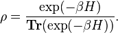
$\rho ={\frac {\exp(-\beta H)}{{\mathbf {Tr}}(\exp(-\beta H))}}.$

For the system to have a ground state, the trace to converge, and the density operator to be generally meaningful, βH must be positive semidefinite. So if hν < μ, and H is negative semidefinite, then β must itself be negative, implying a negative temperature.^[9]

Two-dimensional vortex motion

The two-dimensional systems can exist in negative temperature states.^[10]^[11]

Motional degrees of freedom

Negative temperatures have also been achieved in motional degrees of freedom. Using an optical lattice, upper bounds were placed on the kinetic energy, interaction energy and potential energy of cold 39K atoms. This was done by tuning the interactions of the atoms from repulsive to attractive using a Feshbach resonance and changing the overall harmonic potential from trapping to anti-trapping, thus transforming the Bose-Hubbard Hamiltonian from ${\hat {H}}\rightarrow -{\hat {H}}$ . Performing this transformation adiabatically while keeping the atoms in the Mott insulator regime, it is possible to go from a low entropy positive temperature state to a low entropy negative temperature state. In the negative temperature state, the atoms macroscopically occupy the maximum momentum state of the lattice. The negative temperature ensembles equilibrated and showed long lifetimes in an anti-trapping harmonic potential.^[12]

References

↑ Ramsey, Norman (1956-07-01). "Thermodynamics and Statistical Mechanics at Negative Absolute Temperatures". Physical Review 103 (1): 20–28. Bibcode:1956PhRv..103...20R. doi:10.1103/PhysRev.103.20.
↑ Tremblay, André-Marie (1975-11-18). "Comment on: Negative Kelvin temperatures: some anomalies and a speculation". American Journal of Physics 44 (10): 994–995. Bibcode:1976AmJPh..44..994T. doi:10.1119/1.10248.
↑ Atkins, Peter W. (2010-03-25). The Laws of Thermodynamics: A Very Short Introduction. Oxford University Press. pp. 10–14. ISBN 9780199572199. OCLC 467748903.
↑ Atkins, Peter W. (2010-03-25). The Laws of Thermodynamics: A Very Short Introduction. Oxford University Press. pp. 89–95. ISBN 9780199572199. OCLC 467748903.
↑ Purcell, E. M.; Pound, R. V. (1951-01-15). "A Nuclear Spin System at Negative Temperature". Physical Review 81 (2): 279–280. Bibcode:1951PhRv...81..279P. doi:10.1103/PhysRev.81.279.
↑ Varga, Peter (1998). "Minimax games, spin glasses, and the polynomial-time hierarchy of complexity classes". Physical Review E 57 (6): 6487–6492. arXiv:abs/cond-mat/9604030. Bibcode:1998PhRvE..57.6487V. doi:10.1103/PhysRevE.57.6487.
↑ Ramsey, Norman F. (1998). Spectroscopy with coherent radiation: selected papers of Norman F. Ramsey with commentary. World Scientific series in 20th century physics, v. 21. Singapore; River Edge, N.J.: World Scientific. p. 417. ISBN 9789810232504. OCLC 38753008.
↑ "Positive and negative picokelvin temperatures".
↑ Hsu, W.; Barakat, R. (1992). "Statistics and thermodynamics of luminescent radiation". Physical Review B 46 (11): 6760–6767. Bibcode:1992PhRvB..46.6760H. doi:10.1103/PhysRevB.46.6760.
↑ Montgomery, D.C. (1972). "Two-dimensional vortex motion and "negative temperatures"". Physics Letters A 39 (1): 7–8. Bibcode:1972PhLA...39....7M. doi:10.1016/0375-9601(72)90302-7.
↑ Edwards, S.F.; Taylor, J.B. (1974). "Negative Temperature States of Two-Dimensional Plasmas and Vortex Fluids". Proceedings of the Royal Society of London A 336 (1606): 257–271. Bibcode:1974RSPSA.336..257E. doi:10.1098/rspa.1974.0018. JSTOR 78450.
↑ Braun, S.; Ronzheimer, J. P.; Schreiber, M.; Hodgman, S. S.; Rom, T.; Bloch, I.; Schneider, U. (2013). "Negative Absolute Temperature for Motional Degrees of Freedom". Science 339 (6115): 52–55. doi:10.1126/science.1227831. PMID 23288533.

Kittel, C.; Kroemer, H. (1980). Thermal Physics (2nd ed.). W. H. Freeman. ISBN 0-7167-1088-9.
Castle, J.; Emmerich, W.; Heikes, R.; Miller, R.; Rayne, J. (1965). Science by Degrees: Temperature from Zero to Zero. Walker and Company. LCCN 64023985.

External links

Moriarty, Philip. "−K: Negative Temperatures". Sixty Symbols. Brady Haran for the University of Nottingham.

This article is issued from Wikipedia. The text is available under the Creative Commons Attribution/Share Alike; additional terms may apply for the media files.