Negative frequency

The concept of negative and positive frequency can be as simple as a wheel rotating one way or the other way. A signed value of frequency can indicate both the rate and direction of rotation. The rate is expressed in units such as revolutions (aka cycles) per second (hertz) or radian/second (where 1 cycle corresponds to 2π radians).
Sinusoids
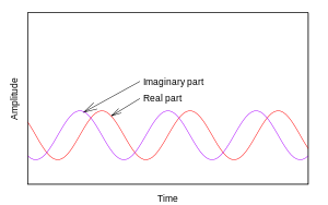
Similar to the rotating vector (Fig 1), the complex-valued function:

exhibits different properties for positive and negative values of the parameter ω. When ω > 0, R(t) appears to lead I(t) by ¼ cycle (= π/2 radians). When ω < 0, the roles are reversed. Fig 2 depicts a negative frequency. R(t) and I(t) are referred to as real and imaginary, respectively. The more-familiar real-valued sinusoid:
-

(Eq.1)
is an analytically more-complicated function than  because it comprises both a negative and positive frequency component. In fact,
  is sometimes called the analytic representation of
  [2] When working with individual, real-valued sinusoids, a negative frequency has an equivalent positive-frequency form; i.e.
  so it is often sufficient to consider every frequency a positive one.
Applications
Perhaps the most well-known application of negative frequency is the calculation:

which is a measure of the amount of frequency ω in the function x(t) over the interval (a,b). When evaluated as a continuous function of ω for the theoretical interval (-∞, ∞), it is known as the Fourier transform of x(t). A brief explanation is that the product of two complex sinusoids is also a complex sinusoid whose frequency is the sum of the original frequencies. So when ω is positive,  causes all the frequencies of x(t) to be reduced by amount ω. Whatever part of x(t) that was at frequency ω is changed to frequency zero, which is just a constant whose amplitude level is a measure of the strength of the original ω content. And whatever part of x(t) that was at frequency zero is changed to a sinusoid at frequency -ω. Similarly, all other frequencies are changed to non-zero values. As the interval (a,b) increases, the contribution of the constant term grows in proportion. But the contributions of the sinusoidal terms only oscillate around zero. So X(ω) improves as a relative measure of the amount of frequency ω in the function x(t).
The Fourier transform of produces a non-zero response only at frequency ω. The transform of  has responses at both ω and -ω, as anticipated by Eq.1.
Sampling of positive and negative frequencies and aliasing

Notes
- ↑ The equivalence is called Euler's formula
- ↑ See Euler's_formula#Relationship_to_trigonometry and Phasor#Addition for examples of calculations simplified by the complex representation.
References
- Positive and Negative Frequencies
- Lyons, Richard G. (Nov 11, 2010). Chapt 8.4. Understanding Digital Signal Processing (3rd ed.). Prentice Hall. 944 pgs. ISBN 0137027419.