Morse potential
| Computational physics |
|---|
 |
|
Numerical analysis · Simulation |
|
Particle |
|
Scientists |
The Morse potential, named after physicist Philip M. Morse, is a convenient model for the potential energy of a diatomic molecule. It is a better approximation for the vibrational structure of the molecule than the QHO (quantum harmonic oscillator) because it explicitly includes the effects of bond breaking, such as the existence of unbound states. It also accounts for the anharmonicity of real bonds and the non-zero transition probability for overtone and combination bands. The Morse potential can also be used to model other interactions such as the interaction between an atom and a surface. Due to its simplicity (only three fitting parameters), it is not used in modern spectroscopy. However, its mathematical form inspired the MLR (Morse/Long-range) potential, first developed by Professor Robert J. Le Roy of University of Waterloo, which is currently the most popular potential energy function used for fitting spectroscopic data.
Potential energy function

The Morse potential energy function is of the form

Here  is the distance between the atoms,
  is the equilibrium bond distance,
  is the well depth (defined relative to the dissociated atoms), and
  controls the 'width' of the potential (the smaller is, the larger the well). The dissociation energy of the bond can be calculated by subtracting the zero point energy
  from the depth of the well. The force constant of the bond can be found by Taylor expansion of
  around
  to the second derivative of the potential energy function, from which it can be shown that the parameter, , is
 ,
,
where  is the force constant at the minimum of the well.
Since the zero of potential energy is arbitrary, the equation for the Morse potential can be rewritten any number of ways by adding or subtracting a constant value. When it is used to model the atom-surface interaction, the energy zero can be redefined so that the Morse potential becomes

which is usually written as

where is now the coordinate perpendicular to the surface. This form approaches zero at infinite and equals  at its minimum, i.e. . It clearly shows that the Morse potential is the combination of a short-range repulsion term (the former) and a long-range attractive term (the latter), analogous to the Lennard-Jones potential.
Vibrational states and energies
Like the quantum harmonic oscillator, the energies and eigenstates of the Morse potential can be found using operator methods.[1] One approach involves applying the factorization method to the Hamiltonian.
To write the stationary states on the Morse potential, i.e. solutions  and
and  of the following Schrödinger equation:
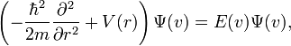
it is convenient to introduce the new variables:

Then, the Schrödinger equation takes the simple form:


Its eigenvalues and eigenstates can be written as:

where
![z=2\lambda e^{{-\left(x-x_{e}\right)}}{\text{; }}N_{n}=n!\left[{\frac {a\left(2\lambda -2n-1\right)}{\Gamma (n+1)\Gamma (2\lambda -n)}}\right]^{{{\frac {1}{2}}}}](/2014-wikipedia_en_all_02_2014/I/media/1/d/d/2/1dd2dd748772fc7bcc77801491ea41d1.png) and
and  is a Laguerre polynomial:

There also exists the following important analytical expression for matrix elements of the coordinate operator (here it is assumed that  and
and  )
[2]
)
[2]

The eigenenergies in the initial variables have form:
![E(v)=h\nu _{0}(v+1/2)-{\frac {\left[h\nu _{0}(v+1/2)\right]^{2}}{4D_{e}}}](/2014-wikipedia_en_all_02_2014/I/media/3/1/6/5/316542e24f3eb81a6dcbad51090b4e87.png)
where  is the vibrational quantum number, and
  has units of frequency, and is mathematically related to the particle mass,
  , and the Morse constants via
 .
.
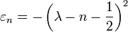
Whereas the energy spacing between vibrational levels in the quantum harmonic oscillator is constant at  , the energy between adjacent levels decreases with increasing in the Morse oscillator. Mathematically, the spacing of Morse levels is
 .
.
This trend matches the anharmonicity found in real molecules. However, this equation fails above some value of  where
where  is calculated to be zero or negative. Specifically,
 .
.
This failure is due to the finite number of bound levels in the Morse potential, and some maximum that remains bound. For energies above , all the possible energy levels are allowed and the equation for is no longer valid.
Below , is a good approximation for the true vibrational structure in non-rotating diatomic molecules. In fact, the real molecular spectra are generally fit to the form1

in which the constants  and
and  can be directly related to the parameters for the Morse potential.
As is clear from dimensional analysis, for historical reasons the last equation uses spectroscopic notation in which represents a wavenumber obeying  , and not an angular frequency given by
  .
.
Morse/Long-range potential
An important extension of the Morse potential that has made the Morse form very useful for modern spectroscopy is the MLR (Morse/Long-range) potential, first developed by Professor Robert J. Le Roy of University of Waterloo. The MLR potential is used as a standard for representing spectroscopic and/or virial data of diatomic molecules by a potential energy curve. It has been used on N2,[3] Ca2,[4] KLi,[5] MgH,[6][7][8] several electronic states of Li2,[9][10][11][12][11][7] Cs2,[13][14] Sr2,[15] ArXe,[7][16] LiCa,[17] LiNa,[18] Br2,[19] Mg2,[20] HF,[21] HCl,[21] HBr,[21] HI,[21] and MgD.[6] More sophisticated versions are used for polyatomic molecules.
See also
References
- 1 CRC Handbook of chemistry and physics, Ed David R. Lide, 87th ed, Section 9, SPECTROSCOPIC CONSTANTS OF DIATOMIC MOLECULES p. 9-82
- Morse, P. M. (1929). "Diatomic molecules according to the wave mechanics. II. Vibrational levels". Phys. Rev. 34. pp. 57–64. Bibcode:1929PhRv...34...57M. doi:10.1103/PhysRev.34.57.
- Girifalco, L. A.; Weizer, G. V. (1959). "Application of the Morse Potential Function to cubic metals". Phys. Rev. 114 (3). p. 687. Bibcode:1959PhRv..114..687G. doi:10.1103/PhysRev.114.687.
- Shore, Bruce W. (1973). "Comparison of matrix methods applied to the radial Schrödinger eigenvalue equation: The Morse potential". J. Chem. Phys. 59 (12). p. 6450. doi:10.1063/1.1680025.
- Keyes, Robert W. (1975). "Bonding and antibonding potentials in group-IV semiconductors". Phys. Rev. Lett. 34 (21). pp. 1334–1337. doi:10.1103/PhysRevLett.34.1334.
- Lincoln, R. C.; Kilowad, K. M.; Ghate, P. B. (1967). "Morse-potential evaluation of second- and third-order elastic constants of some cubic metals". Phys. Rev. 157 (3). pp. 463–466. doi:10.1103/PhysRev.157.463.
- Dong, Shi-Hai; Lemus, R.; Frank, A. (2001). "Ladder operators for the Morse potential". Int. J. Quant. Chem. 86 (5). pp. 433–439. doi:10.1002/qua.10038.
- Zhou, Yaoqi; Karplus, Martin; Ball, Keith D.; Bery, R. Stephen (2002). "The distance fluctuation criterion for melting: Comparison of square-well and Morse Potential models for clusters and homopolymers". J. Chem. Phys 116 (5). pp. 2323–2329. doi:10.1063/1.1426419.
- I.G. Kaplan, in Handbook of Molecular Physics and Quantum Chemistry, Wiley, 2003, p207.
- ↑ F. Cooper, A. Khare, U. Sukhatme, Supersymmetry in Quantum Mechanics, World Scientific, 2001, Table 4.1
- ↑ E. F. Lima and J. E. M. Hornos, "Matrix Elements for the Morse Potential Under an External Field", J. Phys. B: At. Mol. Opt. Phys. 38, pp. 815-825 (2005)
- ↑ Le Roy, R. J.; Y. Huang, C. Jary (2006). "An accurate analytic potential function for ground-state N2 from a direct-potential-fit analysis of spectroscopic data". Journal of Chemical Physics 125: 164310. doi:10.1063/1.2354502.
- ↑ Le Roy, Robert J.; R. D. E. Henderson (2007). "A new potential function form incorporating extended long-range behaviour: application to ground-state Ca2". Molecular Physics 105: 663. doi:10.1080/00268970701241656.
- ↑ Salami, H.; A. J. Ross, P. Crozet, W. Jastrzebski, P. Kowalczyk, R. J. Le Roy (2007). "A full analytic potential energy curve for the a3Σ+ state of KLi from a limited vibrational data set". Journal of Chemical Physics 126: 194313. doi:10.1063/1.2734973.
- ↑ 6.0 6.1 Henderson, R. D. E.; A. Shayesteh, J. Tao, C. Haugen, P. F. Bernath, R. J. Le Roy (4 October 2013). "Accurate Analytic Potential and Born–Oppenheimer Breakdown Functions for MgH and MgD from a Direct-Potential-Fit Data Analysis". The Journal of Physical Chemistry A. doi:10.1021/jp406680r.
- ↑ 7.0 7.1 7.2 Le Roy, R. J.; C. C. Haugen, J. Tao, H. Li (February 2011). "Long-range damping functions improve the short-range behaviour of ‘MLR’ potential energy functions". Molecular Physics 109: 435.
- ↑ Shayesteh, A.; R. D. E. Henderson, R. J. Le Roy, P. F. Bernath (2007). "Ground State Potential Energy Curve and Dissociation Energy of MgH". The Journal of Physical Chemistry A 111: 12495. doi:10.1021/jp075704a.
- ↑ Le Roy, Robert J.; N. S. Dattani, J. A. Coxon, A. J. Ross, Patrick Crozet, C. Linton (25 November 2009). "Accurate analytic potentials for Li2(X) and Li2(A) from 2 to 90 Angstroms, and the radiative lifetime of Li(2p)". Journal of Chemical Physics 131: 204309. doi:10.1063/1.3264688.
- ↑ Dattani, N. S.; R. J. Le Roy (8 May 2013). "A DPF data analysis yields accurate analytic potentials for Li2(a) and Li2(c) that incorporate 3-state mixing near the c-state asymptote". Journal of Molecular Spectroscopy (Special Issue) 268: 199–210. doi:10.1016/j.jms.2011.03.030.
- ↑ 11.0 11.1 W. Gunton, M. Semczuk, N. S. Dattani, K. W. Madison, High resolution photoassociation spectroscopy of the 6Li2 A-state, http://arxiv.org/abs/1309.5870
- ↑ Semczuk, M.; Li, X.; Gunton, W.; Haw, M.; Dattani, N. S.; Witz, J.; Mills, A. K.; Jones, D. J. et al. (2013). "High-resolution photoassociation spectroscopy of the 6Li2 c-state". Phys. Rev. A 87. p. 052505. doi:10.1103/PhysRevA.87.052505.
- ↑ Xie, F.; L. Li, D. Li, V. B. Sovkov, K. V. Minaev, V. S. Ivanov, A. M. Lyyra, S. Magnier (2011). "Joint analysis of the Cs2 a-state and 1 g (33Π1g ) states". Journal of Chemical Physics 135: 02403. doi:10.1063/1.3606397.
- ↑ Coxon, J. A.; P. G. Hajigeorgiou (2010). "The ground X 1Σ+g electronic state of the cesium dimer: Application of a direct potential fitting procedure". Journal of Chemical Physics 132: 094105. doi:10.1063/1.3319739.
- ↑ Stein, A.; H. Knockel, E. Tiemann (April 2010). "The 1S+1S asymptote of Sr2 studied by Fourier-transform spectroscopy". The European Physical Journal D 57 (2): 171–177. doi:10.1140/epjd/e2010-00058-y.
- ↑ Piticco, Lorena; F. Merkt, A. A. Cholewinski, F. R. W. McCourt, R. J. Le Roy (December 2010). "Rovibrational structure and potential energy function of the ground electronic state of ArXe". Journal of Molecular Spectroscopy 264: 83. doi:10.1016/j.jms.2010.08.007.
- ↑ Ivanova, Milena; A. Stein, A. Pashov, A. V. Stolyarov, H. Knockel, E. Tiemann (2011). "The X2Σ+ state of LiCa studied by Fourier-transform spectroscopy". Journal of Chemical Physics 135: 174303. doi:10.1063/1.3652755.
- ↑ Steinke, M.; H. Knockel, E. Tiemann (27 April 2012). "X-state of LiNa studied by Fourier-transform spectroscopy". Physical Review A 85: 042720. doi:10.1103/PhysRevA.85.042720.
- ↑ Yukiya, T.; N. Nishimiya, Y. Samejima, K. Yamaguchi, M. Suzuki, C. D. Boonec, I. Ozier, R. J. Le Roy (January 2013). "Direct-potential-fit analysis for the system of Br2". Journal of Molecular Spectroscopy 283: 32–43. doi:10.1016/j.jms.2012.12.006.
- ↑ Knockel, H.; S. Ruhmann, E. Tiemann (2013). "The X-state of Mg2 studied by Fourier-transform spectroscopy". Journal of Chemical Physics 138: 094303. doi:10.1063/1.4792725.
- ↑ 21.0 21.1 21.2 21.3 Li, Gang; I. E. Gordon, P. G. Hajigeorgiou, J. A. Coxon, L. S. Rothman (July 2013). "Reference spectroscopic data for hydrogen halides, Part II:The line lists". Journal of Quantitative Spectroscopy & Radiative Transfer 130: 284–295. doi:10.1016/j.jqsrt.2013.07.019.