Lyapunov stability

From Wikipedia, the free encyclopedia

This article is about asymptotic stability of nonlinear systems. For stability of linear systems, see exponential stability.

Various types of stability may be discussed for the solutions of differential equations describing dynamical systems. The most important type is that concerning the stability of solutions near to a point of equilibrium. This may be discussed by the theory of Lyapunov. In simple terms, if all solutions of the dynamical system that start out near an equilibrium point $x_{e}$ stay near $x_{e}$ forever, then $x_{e}$ is Lyapunov stable. More strongly, if $x_{e}$ is Lyapunov stable and all solutions that start out near $x_{e}$ converge to $x_{e}$ , then $x_{e}$ is asymptotically stable. The notion of exponential stability guarantees a minimal rate of decay, i.e., an estimate of how quickly the solutions converge. The idea of Lyapunov stability can be extended to infinite-dimensional manifolds, where it is known as structural stability, which concerns the behavior of different but "nearby" solutions to differential equations. Input-to-state stability (ISS) applies Lyapunov notions to systems with inputs.

History

Lyapunov stability is named after Aleksandr Lyapunov, a Russian mathematician who published his book The General Problem of Stability of Motion in 1892.^[1] Lyapunov was the first to consider the modifications necessary in nonlinear systems to the linear theory of stability based on linearizing near a point of equilibrium. His work, initially published in Russian and then translated to French, received little attention for many years. Interest in it started suddenly during the Cold War (1953–1962) period when the so-called "Second Method of Lyapunov" (see below) was found to be applicable to the stability of aerospace guidance systems which typically contain strong nonlinearities not treatable by other methods. A large number of publications appeared then and since in the control and systems literature.^[2]^[3]^[4]^[5]^[6] More recently the concept of the Lyapunov exponent (related to Lyapunov's First Method of discussing stability) has received wide interest in connection with chaos theory. Lyapunov stability methods have also been applied to finding equilibrium solutions in traffic assignment problems.^[7]

Definition for continuous-time systems

Consider an autonomous nonlinear dynamical system

${\dot {x}}=f(x(t)),\;\;\;\;x(0)=x_{0}$ ,

where $x(t)\in {\mathcal {D}}\subseteq {\mathbb {R}}^{n}$ denotes the system state vector, ${\mathcal {D}}$ an open set containing the origin, and $f:{\mathcal {D}}\rightarrow {\mathbb {R}}^{n}$ continuous on ${\mathcal {D}}$ . Suppose $f$ has an equilibrium at $x_{e}$ so that $f(x_{e})=0$ then

This equilibrium is said to be Lyapunov stable, if, for every $\epsilon >0$ , there exists a $\delta =\delta (\epsilon )>0$ such that, if $\|x(0)-x_{e}\|<\delta$ , then $\|x(t)-x_{e}\|<\epsilon$ , for every $t\geq 0$ .
The equilibrium of the above system is said to be asymptotically stable if it is Lyapunov stable and if there exists $\delta >0$ such that if $\|x(0)-x_{e}\|<\delta$ , then $\lim _{{t\rightarrow \infty }}\|x(t)-x_{e}\|=0$ .
The equilibrium of the above system is said to be exponentially stable if it is asymptotically stable and if there exist $\alpha ,\beta ,\delta >0$ such that if $\|x(0)-x_{e}\|<\delta$ , then $\|x(t)-x_{e}\|\leq \alpha \|x(0)-x_{e}\|e^{{-\beta t}}$ , for $t\geq 0$ .

Conceptually, the meanings of the above terms are the following:

Lyapunov stability of an equilibrium means that solutions starting "close enough" to the equilibrium (within a distance $\delta$ from it) remain "close enough" forever (within a distance $\epsilon$ from it). Note that this must be true for any $\epsilon$ that one may want to choose.
Asymptotic stability means that solutions that start close enough not only remain close enough but also eventually converge to the equilibrium.
Exponential stability means that solutions not only converge, but in fact converge faster than or at least as fast as a particular known rate $\alpha \|x(0)-x_{e}\|e^{{-\beta t}}$ .

The trajectory x is (locally) attractive if

$\|y(t)-x(t)\|\rightarrow 0$

for $t\rightarrow \infty$ for all trajectories that start close enough, and globally attractive if this property holds for all trajectories.

That is, if x belongs to the interior of its stable manifold. It is asymptotically stable if it is both attractive and stable. (There are counterexamples showing that attractivity does not imply asymptotic stability. Such examples are easy to create using homoclinic connections.)

Lyapunov's second method for stability

Lyapunov, in his original 1892 work, proposed two methods for demonstrating stability.^[1] The first method developed the solution in a series which was then proved convergent within limits. The second method, which is almost universally used nowadays, makes use of a Lyapunov function V(x) which has an analogy to the potential function of classical dynamics. It is introduced as follows for a system having a point of equilibrium at x=0. Consider a function $V(x):{\mathbb {R}}^{n}\rightarrow {\mathbb {R}}$ such that

$V(x)\geq 0$ with equality if and only if $x=0$ (positive definite)
${\dot {V}}(x)={\frac {d}{dt}}V(x)\leq 0$ with equality if and only if $x=0$ (negative definite).

Then V(x) is called a Lyapunov function candidate and the system is asymptotically stable in the sense of Lyapunov. (Note that $V(0)=0$ is required; otherwise for example $V(x)=1/(1+|x|)$ would "prove" that ${\dot x}(t)=x$ is locally stable. An additional condition called "properness" or "radial unboundedness" is required in order to conclude global asymptotic stability.)

It is easier to visualize this method of analysis by thinking of a physical system (e.g. vibrating spring and mass) and considering the energy of such a system. If the system loses energy over time and the energy is never restored then eventually the system must grind to a stop and reach some final resting state. This final state is called the attractor. However, finding a function that gives the precise energy of a physical system can be difficult, and for abstract mathematical systems, economic systems or biological systems, the concept of energy may not be applicable.

Lyapunov's realization was that stability can be proven without requiring knowledge of the true physical energy, provided a Lyapunov function can be found to satisfy the above constraints.

Definition for discrete-time systems

The definition for discrete-time systems is almost identical to that for continuous-time systems. The definition below provides this, using an alternate language commonly used in more mathematical texts.

Let (X, d) be a metric space and f : X → X a continuous function. A point x in X is said to be Lyapunov stable, if,

$\forall \epsilon >0\ \exists \delta >0\ \forall y\in X\ \left[d(x,y)<\delta \Rightarrow \forall n\in {\mathbf {N}}\ d\left(f^{n}(x),f^{n}(y)\right)<\epsilon \right].$

We say that x is asymptotically stable if it belongs to the interior of its stable set, i.e. if,

$\exists \delta >0\left[d(x,y)<\delta \Rightarrow \lim _{{n\to \infty }}d\left(f^{n}(x),f^{n}(y)\right)=0\right].$

Stability for linear state space models

A linear state space model

${\dot {{\textbf {x}}}}=A{\textbf {x}}$ ,

where $A$ is a finite matrix, is asymptotically stable (in fact, exponentially stable) if all real parts of the eigenvalues of $A$ are negative. This condition is equivalent to the following one:

$A^{{T}}M+MA$

is negative definite for some positive definite matrix $M=M^{{T}}$ . (The relevant Lyapunov function is $V(x)=x^{T}Mx$ .)

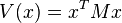Correspondingly, a time-discrete linear state space model

${{\textbf {x}}_{{t+1}}}=A{\textbf {x}}_{t}$

is asymptotically stable (in fact, exponentially stable) if all the eigenvalues of $A$ have a modulus smaller than one.

This latter condition has been generalized to switched systems: a linear switched discrete time system (ruled by a set of matrices $\{A_{1},\dots ,A_{m}\}$ )

${{\textbf {x}}_{{t+1}}}=A_{{i_{t}}}{\textbf {x}}_{t},\quad A_{{i_{t}}}\in \{A_{1},\dots ,A_{m}\}$

is asymptotically stable (in fact, exponentially stable) if the joint spectral radius of the set $\{A_{1},\dots ,A_{m}\}$ is smaller than one.

Stability for systems with inputs

A system with inputs (or controls) has the form

${\dot {{\textbf {x}}}}={\textbf {f(x,u)}}$

where the (generally time-dependent) input u(t) may be viewed as a control, external input, stimulus, disturbance, or forcing function. The study of such systems is the subject of control theory and applied in control engineering. For systems with inputs, one must quantify the effect of inputs on the stability of the system. The main two approaches to this analysis are BIBO stability (for linear systems) and input-to-state (ISS) stability (for nonlinear systems)

Example

Consider an equation, where compared to the Van der Pol oscillator equation the friction term is changed:

${\ddot {y}}+y-\varepsilon \left({\frac {{\dot {y}}^{{3}}}{3}}-{\dot {y}}\right)=0.$

The equilibrium is at : ${\ddot {y}}=y=0.$

Here is a good example of an unsuccessful try to find a Lyapunov function that proves stability:

Let

$x_{{1}}=y,x_{{2}}={\dot {y}}$

so that the corresponding system is

${\dot {x_{{2}}}}=-x_{{1}}+\varepsilon \left({\frac {{x_{{2}}}^{{3}}}{3}}-{x_{{2}}}\right).$

Let us choose as a Lyapunov function

$V={\frac {1}{2}}\left(x_{{1}}^{{2}}+x_{{2}}^{{2}}\right)$

which is clearly positive definite. Its derivative is

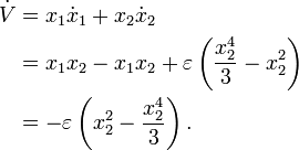
${\begin{aligned}{\dot {V}}&=x_{{1}}{\dot x}_{{1}}+x_{{2}}{\dot x}_{{2}}\\&=x_{{1}}x_{{2}}-x_{{1}}x_{{2}}+\varepsilon \left({\frac {x_{{2}}^{4}}{3}}-{x_{{2}}^{2}}\right)\\&=-\varepsilon \left({x_{{2}}^{2}}-{\frac {x_{{2}}^{4}}{3}}\right).\end{aligned}}$

It seems that if the parameter $\varepsilon$ is positive, stability is asymptotic for $x_{{2}}^{{2}}<3.$ But this is wrong, since ${\dot {V}}$ does not depend on $x_{1}$ , and will be 0 everywhere on the $x_{1}$ axis.

Barbalat's lemma and stability of time-varying systems

Assume that f is function of time only.

Having ${\dot {f}}(t)\to 0$ does not imply that $f(t)$ has a limit at $t\to \infty$ . For example, $f(t)=\sin(\ln(t)),\;t>0$ .
Having $f(t)$ approaching a limit as $t\to \infty$ does not imply that ${\dot {f}}(t)\to 0$ . For example, $f(t)=\sin(t^{2})/t,\;t>0$ .
Having $f(t)$ lower bounded and decreasing ( ${\dot {f}}\leq 0$ ) implies it converges to a limit. But it does not say whether or not ${\dot {f}}\to 0$ as $t\to \infty$ .

Barbalat's Lemma says:

If $f(t)$ has a finite limit as $t\to \infty$ and if ${\dot {f}}$ is uniformly continuous (or ${\ddot {f}}$ is bounded), then ${\dot {f}}(t)\to 0$ as $t\to \infty$ .

Usually, it is difficult to analyze the asymptotic stability of time-varying systems because it is very difficult to find Lyapunov functions with a negative definite derivative.

We know that in case of autonomous (time-invariant) systems, if ${\dot {V}}$ is negative semi-definite (NSD), then also, it is possible to know the asymptotic behaviour by invoking invariant-set theorems. However, this flexibility is not available for time-varying systems. This is where "Barbalat's lemma" comes into picture. It says:

IF $V(x,t)$ satisfies following conditions:

$V(x,t)$ is lower bounded
${\dot {V}}(x,t)$ is negative semi-definite (NSD)
${\dot {V}}(x,t)$ is uniformly continuous in time (satisfied if ${\ddot {V}}$ is finite)

then ${\dot {V}}(x,t)\to 0$ as $t\to \infty$ .

The following example is taken from page 125 of Slotine and Li's book Applied Nonlinear Control.

Consider a non-autonomous system

${\dot {e}}=-e+g\cdot w(t)$

${\dot {g}}=-e\cdot w(t).$

This is non-autonomous because the input $w$ is a function of time. Assume that the input $w(t)$ is bounded.

Taking $V=e^{2}+g^{2}$ gives ${\dot {V}}=-2e^{2}\leq 0.$

This says that $V(t)<=V(0)$ by first two conditions and hence $e$ and $g$ are bounded. But it does not say anything about the convergence of $e$ to zero. Moreover, the invariant set theorem cannot be applied, because the dynamics is non-autonomous.

Using Barbalat's lemma:

${\ddot {V}}=-4e(-e+g\cdot w)$ .

This is bounded because $e$ , $g$ and $w$ are bounded. This implies ${\dot {V}}\to 0$ as $t\to \infty$ and hence $e\to 0$ . This proves that the error converges.

References

↑ 1.0 1.1 Lyapunov A. M. The General Problem of the Stability of Motion (In Russian), Doctoral dissertation, Univ. Kharkov 1892 English translations: (1) Stability of Motion, Academic Press, New-York & London, 1966 (2) The General Problem of the Stability of Motion, (A. T. Fuller trans.) Taylor & Francis, London 1992. Included is a biography by Smirnov and an extensive bibliography of Lyapunov's work.
↑ Letov A.M. Stability of Nonlinear Control Systems (Russian) Moscow 1955 (Gostekhizdat); English tr. Princeton 1961
↑ Kalman R. E. & Bertram J. F: "Control System Analysis and Design via the Second Method of Lyapunov", J. Basic Engrg vol.88 1960 pp.371; 394
↑ LaSalle J. P. & Lefschetz S.: Stability by Lyapunov's Second Method with Applications, New York 1961 (Academic)
↑ Parks P.C: "Liapunov's method in automatic control theory", Control I Nov 1962 II Dec 1962
↑ Kalman R.E. "Lyapunov functions for the problem of Lurie in automatic control", Proc Nat Acad.Sci USA, Feb 1963, 49, no.2,201-.
↑ Smith M.J. and Wisten M.B., A continuous day-to-day traffic assignment model and the existence of a continuous dynamic user equilibrium , Annals of Operations Research, Volume 60, 1995

External links

http://www.mne.ksu.edu/research/laboratories/non-linear-controls-lab (login required)

This article incorporates material from asymptotically stable on PlanetMath, which is licensed under the Creative Commons Attribution/Share-Alike License.

This article is issued from Wikipedia. The text is available under the Creative Commons Attribution/Share Alike; additional terms may apply for the media files.