Kernel (statistics)

From Wikipedia, the free encyclopedia

The term kernel has two separate meanings in statistics.

In Bayesian statistics

In statistics, especially in Bayesian statistics, the kernel of a probability density function (pdf) or probability mass function (pmf) is the form of the pdf or pmf in which any factors that are not functions of any of the variables in the domain are omitted.^{[citation needed]} Note that such factors may well be functions of the parameters of the pdf or pmf. These factors form part of the normalization factor of the probability distribution, and are unnecessary in many situations. For example, in pseudo-random number sampling, most sampling algorithms ignore the normalization factor. In addition, in Bayesian analysis of conjugate prior distributions, the normalization factors are generally ignored during the calculations, and only the kernel considered. At the end, the form of the kernel is examined, and if it matches a known distribution, the normalization factor can be reinstated. Otherwise, it may be unnecessary (for example, if the distribution only needs to be sampled from).

For many distributions, the kernel can be written in closed form, but not the normalization constant.

An example is the normal distribution. Its probability density function is

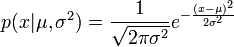
$p(x|\mu ,\sigma ^{2})={\frac {1}{{\sqrt {2\pi \sigma ^{2}}}}}e^{{-{\frac {(x-\mu )^{2}}{2\sigma ^{2}}}}}$

and the associated kernel is

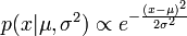
$p(x|\mu ,\sigma ^{2})\propto e^{{-{\frac {(x-\mu )^{2}}{2\sigma ^{2}}}}}$

Note that the factor in front of the exponential has been omitted, even though it contains the parameter $\sigma ^{2}$ , because it is not a function of the domain variable $x$ .

In non-parametric statistics

In non-parametric statistics, a kernel is a weighting function used in non-parametric estimation techniques. Kernels are used in kernel density estimation to estimate random variables' density functions, or in kernel regression to estimate the conditional expectation of a random variable. Kernels are also used in time-series, in the use of the periodogram to estimate the spectral density. An additional use is in the estimation of a time-varying intensity for a point process.

Commonly, kernel widths must also be specified when running a non-parametric estimation.

Definition

A kernel is a non-negative real-valued integrable function K satisfying the following two requirements:

$\int _{{-\infty }}^{{+\infty }}K(u)\,du=1\,;$
$K(-u)=K(u){\mbox{ for all values of }}u\,.$

The first requirement ensures that the method of kernel density estimation results in a probability density function. The second requirement ensures that the average of the corresponding distribution is equal to that of the sample used.

If K is a kernel, then so is the function K* defined by K*(u) = λK(λu), where λ > 0. This can be used to select a scale that is appropriate for the data.

Kernel functions in common use

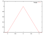
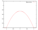
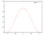
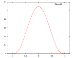
Several types of kernel functions are commonly used: uniform, triangle, Epanechnikov,^[1] quartic (biweight), tricube,^[2] triweight, Gaussian,quadratic^[3] and cosine.

In the table below, 1_{…} is the indicator function.

Kernel Functions, K(u)		$\textstyle \int u^{2}K(u)du$	$\textstyle \int K^{2}(u)du$
Uniform	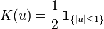$K(u)={\frac 12}\,{\mathbf {1}}_{{\{\|u\|\leq 1\}}}$	${\frac 13}$	${\frac 12}$
Triangular	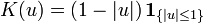$K(u)=(1-\|u\|)\,{\mathbf {1}}_{{\{\|u\|\leq 1\}}}$	${\frac {1}{6}}$	${\frac {2}{3}}$
Epanechnikov	$K(u)={\frac {3}{4}}(1-u^{2})\,{\mathbf {1}}_{{\{\|u\|\leq 1\}}}$	${\frac {1}{5}}$	${\frac {3}{5}}$
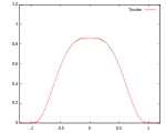
Quartic (biweight)	$K(u)={\frac {15}{16}}(1-u^{2})^{2}\,{\mathbf {1}}_{{\{\|u\|\leq 1\}}}$	${\frac {1}{7}}$	${\frac {5}{7}}$
Triweight	$K(u)={\frac {35}{32}}(1-u^{2})^{3}\,{\mathbf {1}}_{{\{\|u\|\leq 1\}}}$	${\frac {1}{9}}$	${\frac {350}{429}}$
Tricube	$K(u)={\frac {70}{81}}(1-{\left\|u\right\|}^{3})^{3}\,{\mathbf {1}}_{{\{\|u\|\leq 1\}}}$	${\frac {35}{243}}$	${\frac {175}{247}}$
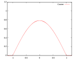
Gaussian	$K(u)={\frac {1}{{\sqrt {2\pi }}}}e^{{-{\frac {1}{2}}u^{2}}}$	$1\,$	${\frac {1}{2{\sqrt \pi }}}$
Cosine	$K(u)={\frac {\pi }{4}}\cos \left({\frac {\pi }{2}}u\right){\mathbf {1}}_{{\{\|u\|\leq 1\}}}$	$1-{\frac {8}{\pi ^{2}}}$	${\frac {\pi ^{2}}{16}}$
Logistic	$K(u)={\frac {1}{e^{{u}}+2+e^{{-u}}}}$	${\frac {\pi ^{2}}{3}}$	${\frac {1}{6}}$

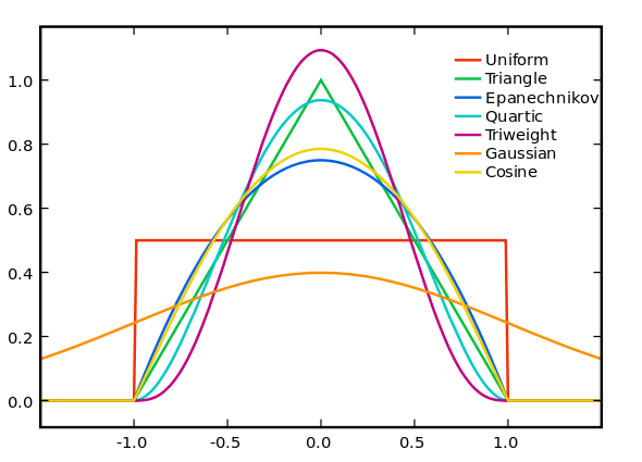
All of the above Kernels in a Common Coordinate System

References

↑ Named for Epanechnikov, V. A. (1969). "Non-Parametric Estimation of a Multivariate Probability Density". Theory Probab. Appl. 14 (1): 153–158. doi:10.1137/1114019.
↑ Altman, N. S. (1992). "An introduction to kernel and nearest neighbor nonparametric regression". The American Statistician 46 (3): 175–185.
↑ Cleveland, W. S. & Devlin, S. J. (1988). "Locally weighted regression: An approach to regression analysis by local fitting". Journal of the American Statistical Association 83: 596–610.

Li, Qi; Racine, Jeffrey S. (2007). Nonparametric Econometrics: Theory and Practice. Princeton University Press. ISBN 0-691-12161-3. Cite uses deprecated parameters (help)

Zucchini, Walter. "APPLIED SMOOTHING TECHNIQUES Part 1: Kernel Density Estimation". Retrieved 28 March 2012.

Comaniciu, D; Meer, P (2002). "Mean shift: A robust approach toward feature space analysis". IEEE Transactions on Pattern Analysis and Machine Intelligence 24 (5): 603–619. doi:10.1109/34.1000236. CiteSeerX: 10.1.1.76.8968.

This article is issued from Wikipedia. The text is available under the Creative Commons Attribution/Share Alike; additional terms may apply for the media files.