Hurwitz zeta function

From Wikipedia, the free encyclopedia

In mathematics, the Hurwitz zeta function, named after Adolf Hurwitz, is one of the many zeta functions. It is formally defined for complex arguments s with Re(s) > 1 and q with Re(q) > 0 by

$\zeta (s,q)=\sum _{{n=0}}^{\infty }{\frac {1}{(q+n)^{{s}}}}.$

This series is absolutely convergent for the given values of s and q and can be extended to a meromorphic function defined for all s≠1. The Riemann zeta function is ζ(s,1).

Analytic continuation

If Re(s) ≤ 1 the Hurwitz zeta function can be defined by the equation

$\zeta (s,q)=\Gamma (1-s){\frac {1}{2\pi i}}\int _{C}{\frac {z^{{s-1}}e^{{qz}}}{1-e^{z}}}dz$

where the contour C is a loop around the negative real axis. This provides an analytic continuation of $\zeta (s,q)$ .

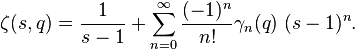
The Hurwitz zeta function can be extended by analytic continuation to a meromorphic function defined for all complex numbers s with s ≠ 1. At s = 1 it has a simple pole with residue 1. The constant term is given by

$\lim _{{s\to 1}}\left[\zeta (s,q)-{\frac {1}{s-1}}\right]={\frac {-\Gamma '(q)}{\Gamma (q)}}=-\psi (q)$

where Γ is the Gamma function and ψ is the digamma function.

Series representation

A convergent series representation defined for (real) q > 0 and any complex s ≠ 1 was given by Helmut Hasse in 1930:^[1]

$\zeta (s,q)={\frac {1}{s-1}}\sum _{{n=0}}^{\infty }{\frac {1}{n+1}}\sum _{{k=0}}^{n}(-1)^{k}{n \choose k}(q+k)^{{1-s}}.$

This series converges uniformly on compact subsets of the s-plane to an entire function. The inner sum may be understood to be the nth forward difference of $q^{{1-s}}$ ; that is,

$\Delta ^{n}q^{{1-s}}=\sum _{{k=0}}^{n}(-1)^{{n-k}}{n \choose k}(q+k)^{{1-s}}$

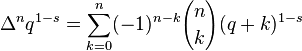
where Δ is the forward difference operator. Thus, one may write

${\begin{aligned}\zeta (s,q)&={\frac {1}{s-1}}\sum _{{n=0}}^{\infty }{\frac {(-1)^{n}}{n+1}}\Delta ^{n}q^{{1-s}}\\&={\frac {1}{s-1}}{\log(1+\Delta ) \over \Delta }q^{{1-s}}\end{aligned}}$

Integral representation

The function has an integral representation in terms of the Mellin transform as

$\zeta (s,q)={\frac {1}{\Gamma (s)}}\int _{0}^{\infty }{\frac {t^{{s-1}}e^{{-qt}}}{1-e^{{-t}}}}dt$

for $\Re s>1$ and $\Re q>0.$

Hurwitz's formula

Hurwitz's formula is the theorem that

$\zeta (1-s,x)={\frac {1}{2s}}\left[e^{{-i\pi s/2}}\beta (x;s)+e^{{i\pi s/2}}\beta (1-x;s)\right]$

where

$\beta (x;s)=2\Gamma (s+1)\sum _{{n=1}}^{\infty }{\frac {\exp(2\pi inx)}{(2\pi n)^{s}}}={\frac {2\Gamma (s+1)}{(2\pi )^{s}}}{\mbox{Li}}_{s}(e^{{2\pi ix}})$

is a representation of the zeta that is valid for $0\leq x\leq 1$ and s > 1. Here, ${\text{Li}}_{s}(z)$ is the polylogarithm.

Functional equation

The functional equation relates values of the zeta on the left- and right-hand sides of the complex plane. For integers $1\leq m\leq n$ ,

$\zeta \left(1-s,{\frac {m}{n}}\right)={\frac {2\Gamma (s)}{(2\pi n)^{s}}}\sum _{{k=1}}^{n}\left[\cos \left({\frac {\pi s}{2}}-{\frac {2\pi km}{n}}\right)\;\zeta \left(s,{\frac {k}{n}}\right)\right]$

holds for all values of s.

Taylor series

The derivative of the zeta in the second argument is a shift:

${\frac {\partial }{\partial q}}\zeta (s,q)=-s\zeta (s+1,q).$

Thus, the Taylor series has the distinctly umbral form:

$\zeta (s,x+y)=\sum _{{k=0}}^{\infty }{\frac {y^{k}}{k!}}{\frac {\partial ^{k}}{\partial x^{k}}}\zeta (s,x)=\sum _{{k=0}}^{\infty }{s+k-1 \choose s-1}(-y)^{k}\zeta (s+k,x).$

Alternatively,

$\zeta (s,q)={\frac {1}{q^{s}}}+\sum _{{n=0}}^{{\infty }}(-q)^{n}{s+n-1 \choose n}\zeta (s+n),$

with $|q|<1$ .^[2]

Closely related is the Stark–Keiper formula:

$\zeta (s,N)=\sum _{{k=0}}^{\infty }\left[N+{\frac {s-1}{k+1}}\right]{s+k-1 \choose s-1}(-1)^{k}\zeta (s+k,N)$

which holds for integer N and arbitrary s. See also Faulhaber's formula for a similar relation on finite sums of powers of integers.

Laurent series

The Laurent series expansion can be used to define Stieltjes constants that occur in the series

$\zeta (s,q)={\frac {1}{s-1}}+\sum _{{n=0}}^{\infty }{\frac {(-1)^{n}}{n!}}\gamma _{n}(q)\;(s-1)^{n}.$

Specifically $\gamma _{0}(q)=-\psi (q)$ and $\gamma _{0}(1)=-\psi (1)=\gamma _{0}=\gamma$ .

Fourier transform

The discrete Fourier transform of the Hurwitz zeta function with respect to the order s is the Legendre chi function.

Relation to Bernoulli polynomials

The function $\beta$ defined above generalizes the Bernoulli polynomials:

$B_{n}(x)=-\Re \left[(-i)^{n}\beta (x;n)\right]$

where $\Re z$ denotes the real part of z. Alternately,

$\zeta (-n,x)=-{B_{{n+1}}(x) \over n+1}.$

In particular, the relation holds for $n=0$ and one has

$\zeta (0,x)={\frac {1}{2}}-x.$

Relation to Jacobi theta function

If $\vartheta (z,\tau )$ is the Jacobi theta function, then

$\int _{0}^{\infty }\left[\vartheta (z,it)-1\right]t^{{s/2}}{\frac {dt}{t}}=\pi ^{{-(1-s)/2}}\Gamma \left({\frac {1-s}{2}}\right)\left[\zeta (1-s,z)+\zeta (1-s,1-z)\right]$

holds for $\Re s>0$ and z complex, but not an integer. For z=n an integer, this simplifies to

$\int _{0}^{\infty }\left[\vartheta (n,it)-1\right]t^{{s/2}}{\frac {dt}{t}}=2\ \pi ^{{-(1-s)/2}}\ \Gamma \left({\frac {1-s}{2}}\right)\zeta (1-s)=2\ \pi ^{{-s/2}}\ \Gamma \left({\frac {s}{2}}\right)\zeta (s).$

where ζ here is the Riemann zeta function. Note that this latter form is the functional equation for the Riemann zeta function, as originally given by Riemann. The distinction based on z being an integer or not accounts for the fact that the Jacobi theta function converges to the Dirac delta function in z as $t\rightarrow 0$ .

Relation to Dirichlet L-functions

At rational arguments the Hurwitz zeta function may be expressed as a linear combination of Dirichlet L-functions and vice versa: The Hurwitz zeta function coincides with Riemann's zeta function ζ(s) when q = 1, when q = 1/2 it is equal to (2^s−1)ζ(s),^[3] and if q = n/k with k > 2, (n,k) > 1 and 0 < n < k, then^[4]

$\zeta (s,n/k)={\frac {k^{s}}{\varphi (k)}}\sum _{\chi }\overline {\chi }(n)L(s,\chi ),$

the sum running over all Dirichlet characters mod k. In the opposite direction we have the linear combination^[3]

$L(s,\chi )={\frac {1}{k^{s}}}\sum _{{n=1}}^{k}\chi (n)\;\zeta \left(s,{\frac {n}{k}}\right).$

There is also the multiplication theorem

$k^{s}\zeta (s)=\sum _{{n=1}}^{k}\zeta \left(s,{\frac {n}{k}}\right),$

of which a useful generalization is the distribution relation^[5]

$\sum _{{p=0}}^{{q-1}}\zeta (s,a+p/q)=q^{s}\,\zeta (s,qa).$

(This last form is valid whenever q a natural number and 1 − qa is not.)

Zeros

If q=1 the Hurwitz zeta function reduces to the Riemann zeta function itself; if q=1/2 it reduces to the Riemann zeta function multiplied by a simple function of the complex argument s (vide supra), leading in each case to the difficult study of the zeros of Riemann's zeta function. In particular, there will be no zeros with real part greater than or equal to 1. However, if 0<q<1 and q≠1/2, then there are zeros of Hurwitz's zeta function in the strip 1<Re(s)<1+ε for any positive real number ε. This was proved by Davenport and Heilbronn for rational and non-algebraic irrational q,^[6] and by Cassels for algebraic irrational q.^[7]^[3]

Rational values

The Hurwitz zeta function occurs in a number of striking identities at rational values.^[8] In particular, values in terms of the Euler polynomials $E_{n}(x)$ :

$E_{{2n-1}}\left({\frac {p}{q}}\right)=(-1)^{n}{\frac {4(2n-1)!}{(2\pi q)^{{2n}}}}\sum _{{k=1}}^{q}\zeta \left(2n,{\frac {2k-1}{2q}}\right)\cos {\frac {(2k-1)\pi p}{q}}$

and

$E_{{2n}}\left({\frac {p}{q}}\right)=(-1)^{n}{\frac {4(2n)!}{(2\pi q)^{{2n+1}}}}\sum _{{k=1}}^{q}\zeta \left(2n+1,{\frac {2k-1}{2q}}\right)\sin {\frac {(2k-1)\pi p}{q}}$

One also has

$\zeta \left(s,{\frac {2p-1}{2q}}\right)=2(2q)^{{s-1}}\sum _{{k=1}}^{q}\left[C_{s}\left({\frac {k}{q}}\right)\cos \left({\frac {(2p-1)\pi k}{q}}\right)+S_{s}\left({\frac {k}{q}}\right)\sin \left({\frac {(2p-1)\pi k}{q}}\right)\right]$

which holds for $1\leq p\leq q$ . Here, the $C_{\nu }(x)$ and $S_{\nu }(x)$ are defined by means of the Legendre chi function $\chi _{\nu }$ as

$C_{\nu }(x)=\operatorname {Re}\,\chi _{\nu }(e^{{ix}})$

and

$S_{\nu }(x)=\operatorname {Im}\,\chi _{\nu }(e^{{ix}}).$

For integer values of ν, these may be expressed in terms of the Euler polynomials. These relations may be derived by employing the functional equation together with Hurwitz's formula, given above.

Applications

Hurwitz's zeta function occurs in a variety of disciplines. Most commonly, it occurs in number theory, where its theory is the deepest and most developed. However, it also occurs in the study of fractals and dynamical systems. In applied statistics, it occurs in Zipf's law and the Zipf–Mandelbrot law. In particle physics, it occurs in a formula by Julian Schwinger,^[9] giving an exact result for the pair production rate of a Dirac electron in a uniform electric field.

Special cases and generalizations

The Hurwitz zeta function with non-negative integer m is related to the polygamma function:

$\psi ^{{(m)}}(z)=(-1)^{{m+1}}m!\zeta (m+1,z)\ .$

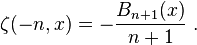
For negative integer −n the values are related to the Bernoulli polynomials:^[10]

$\zeta (-n,x)=-{\frac {B_{{n+1}}(x)}{n+1}}\ .$

The Barnes zeta function generalizes the Hurwitz zeta function.

The Lerch transcendent generalizes the Hurwitz zeta:

$\Phi (z,s,q)=\sum _{{k=0}}^{\infty }{\frac {z^{k}}{(k+q)^{s}}}$

and thus

$\zeta (s,q)=\Phi (1,s,q).\,$

Hypergeometric function

$\zeta (s,a)=a^{{-s}}\cdot {}_{{s+1}}F_{s}(1,a_{1},a_{2},\ldots a_{s};a_{1}+1,a_{2}+1,\ldots a_{s}+1;1)$ where $a_{1}=a_{2}=\ldots =a_{s}=a{\text{ and }}a\notin \mathbb{N} {\text{ and }}s\in \mathbb{N} ^{+}.$

Meijer G-function

$\zeta (s,a)=G\,_{{s+1,\,s+1}}^{{\,1,\,s+1}}\left(-1\;\left|\;{\begin{matrix}0,1-a,\ldots ,1-a\\0,-a,\ldots ,-a\end{matrix}}\right)\right.\qquad \qquad s\in \mathbb{N} ^{+}.$

Notes

↑ Hasse, Helmut (1930), "Ein Summierungsverfahren für die Riemannsche ζ-Reihe", Mathematische Zeitschrift 32 (1): 458–464, doi:10.1007/BF01194645
↑ Vepstas, Linas (2007). "An efficient algorithm for accelerating the convergence of oscillatory series, useful for computing the polylogarithm and Hurwitz zeta functions". arXiv:math/0702243.
↑ 3.0 3.1 3.2 Davenport (1967) p.73
↑ Lowry, David. "Hurwitz Zeta is a sum of Dirichlet L functions, and vice-versa". mixedmath. Retrieved 8 February 2013.
↑ Kubert, Daniel S.; Lang, Serge (1981). Modular Units. Grundlehren der Mathematischen Wissenschaften 244. Springer-Verlag. p. 13. ISBN 0-387-90517-0. Zbl 0492.12002.
↑ Davenport, H. & Heilbronn, H. (1936), "On the zeros of certain Dirichlet series", Journal of the London Mathematical Society 11 (3): 181–185, doi:10.1112/jlms/s1-11.3.181
↑ Cassels, J. W. S. (1961), "Footnote to a note of Davenport and Heilbronn", Journal of the London Mathematical Society 36 (1): 177–184, doi:10.1112/jlms/s1-36.1.177
↑ Given by Cvijović, Djurdje & Klinowski, Jacek (1999), "Values of the Legendre chi and Hurwitz zeta functions at rational arguments", Mathematics of Computation 68 (228): 1623–1630, Bibcode:1999MaCom..68.1623C, doi:10.1090/S0025-5718-99-01091-1
↑ Schwinger, J. (1951), "On gauge invariance and vacuum polarization", Physical Review 82 (5): 664–679, Bibcode:1951PhRv...82..664S, doi:10.1103/PhysRev.82.664
↑ Apostol (1976) p.264

References

Apostol, T. M. (2010), "Hurwitz zeta function", in Olver, Frank W. J.; Lozier, Daniel M.; Boisvert, Ronald F.; Clark, Charles W., NIST Handbook of Mathematical Functions, Cambridge University Press, ISBN 978-0521192255, MR 2723248
See chapter 12 of Apostol, Tom M. (1976), Introduction to analytic number theory, Undergraduate Texts in Mathematics, New York-Heidelberg: Springer-Verlag, ISBN 978-0-387-90163-3, MR 0434929, Zbl 0335.10001
Milton Abramowitz and Irene A. Stegun, Handbook of Mathematical Functions, (1964) Dover Publications, New York. ISBN 0-486-61272-4. (See Paragraph 6.4.10 for relationship to polygamma function.)
Davenport, Harold (1967). Multiplicative number theory. Lectures in advanced mathematics 1. Chicago: Markham. Zbl 0159.06303.
Miller, Jeff; Adamchik, Victor S. (1998). "Derivatives of the Hurwitz Zeta Function for Rational Arguments". Journal of Computational and Applied Mathematics 100: 201–206. doi:10.1016/S0377-0427(98)00193-9.
Vepstas, Linas. "The Bernoulli Operator, the Gauss–Kuzmin–Wirsing Operator, and the Riemann Zeta".
Mező, István; Dil, Ayhan (2010). "Hyperharmonic series involving Hurwitz zeta function". Journal of Number Theory 130 (2): 360–369. doi:10.1016/j.jnt.2009.08.005.

External links

Jonathan Sondow and Eric W. Weisstein, "Hurwitz Zeta Function", MathWorld.

This article is issued from Wikipedia. The text is available under the Creative Commons Attribution/Share Alike; additional terms may apply for the media files.