Gröbner basis

From Wikipedia, the free encyclopedia

In mathematics, and more specifically in computer algebra, computational algebraic geometry, and computational commutative algebra, a Gröbner basis is a particular kind of generating set of an ideal in a polynomial ring over a field K[x₁, ..,x_n]. A Gröbner basis allows many important properties of the ideal and the associated algebraic variety to be deduced easily, such as the dimension and the number of zeros when it is finite. Gröbner basis computation is one of the main practical tools for solving systems of polynomial equations and computing the images of algebraic varieties under projections or rational maps.

Gröbner basis computation can be seen as a multivariate, non-linear generalization of both Euclid's algorithm for computing polynomial greatest common divisors, and Gaussian elimination for linear systems.^[1]

Gröbner bases were introduced in 1965, together with an algorithm to compute them (Buchberger's algorithm), by Bruno Buchberger in his Ph.D. thesis. He named them after his advisor Wolfgang Gröbner. In 2007, Buchberger received the Association for Computing Machinery's Paris Kanellakis Theory and Practice Award for this work. An analogous concept for local rings was developed independently by Heisuke Hironaka in 1964, who named them standard bases.

The theory of Gröbner bases has been extended by many authors in various directions. It has been generalized to other structures such as polynomials over principal ideal rings or polynomial rings, and also some classes of non-commutative rings and algebras.

Background

Polynomial ring

Main article: Polynomial ring

Gröbner bases are primarily defined for ideals in a polynomial ring $R=K[x_{1},\ldots ,x_{n}]$ over a field $K$ . Although the theory works for any field, most Gröbner basis computations are done either when $K$ is the field of rationals or the integers modulo a prime number.

A polynomial is a sum $c_{1}M_{1}+\cdots +c_{m}M_{m}$ where the $c_{i}$ are nonzero elements of $K$ and the $M_{i}$ are monomials or "power products" of the variables. This means that a monomial $M$ is a product $M=x_{1}^{{a_{1}}}\cdots x_{n}^{{a_{n}}},$ where the $a_{i}$ are nonnegative integers. The vector $A=[a_{1},\ldots ,a_{n}]$ is called the exponent vector of $M$ . The notation is often abbreviated as $x_{1}^{{a_{1}}}\cdots x_{n}^{{a_{n}}}=X^{A}$ . Monomials are uniquely defined by their exponent vectors so computers can represent monomials efficiently as exponent vectors, and polynomials as lists of exponent vectors and their coefficients.

If $F=\{f_{1},\ldots ,f_{k}\}$ is a finite set of polynomials in a polynomial ring $R$ , the ideal generated by $F$ is

$\langle f_{1},\ldots ,f_{k}\rangle =\left\{\sum _{{i=1}}^{k}g_{i}f_{i}\;|\;g_{1},\ldots ,g_{k}\in K[x_{1},\ldots ,x_{n}]\right\}.$

Monomial ordering

Main article: Monomial order

All operations related to Gröbner bases require the choice of a total order on the monomials, with the following properties of compatibility with multiplication. For all monomials $M$ , $N$ , $P$ ,

$M<N\Longleftrightarrow MP<NP$
$M<MP$ .

A total order satisfying these condition is sometimes called an admissible ordering.

These conditions imply Noetherianity, which means that every strictly decreasing sequence of monomials is finite.

Although Gröbner basis theory does not depend on a particular choice of an admissible monomial ordering, three monomial orderings are specially important for the applications:

Lexicographical ordering, commonly called lex or plex (for pure lexical ordering).
Total degree reverse lexicographical ordering, commonly called degrevlex.
Elimination ordering, lexdeg.

Gröbner basis theory was initially introduced for the lexicographical ordering. It was soon realised that the Gröbner basis for degrevlex is almost always much easier to compute, and that it is almost always easier to compute a lex Gröbner basis by first computing the degrevlex basis and then using a "change of ordering algorithm". When elimination is needed, degrevlex is not convenient; both lex and lexdeg may be used but, again, many computations are relatively easy with lexdeg and almost impossible with lex.

Once a monomial ordering is fixed, the terms of a polynomial (product of a monomial with its nonzero coefficient) are naturally ordered by decreasing monomials (for this order). This makes the representation of a polynomial as an ordered list of pairs coefficient–exponent vector a canonical representation of the polynomials. The first (greatest) term of a polynomial $p$ for this ordering and the corresponding monomial and coefficient are respectively called the leading term, leading monomial and leading coefficient and denoted, in this article, lt( $p$ ), lm( $p$ ) and lc( $p$ ).

Reduction

The concept of reduction, also called multivariate division or normal form computation, is central to Gröbner basis theory. It is a multivariate generalization of the Euclidean division of univariate polynomials.

In this section we suppose a fixed monomial ordering, which will not be defined explicitly.

Given two polynomials f and g, one says that f is reducible by g if some monomial m in f is a multiple of the leading monomial lm(g) of g. If m happens to be the leading monomial of f then one says that f is lead-reducible by g. If c is the coefficient of m in f and m = q lm(g), the one-step reduction of f by g is the operation that associates to f the polynomial

$\operatorname {red}_{1}(f,g)=f-{\frac {c}{\operatorname {lc}(g)}}\,q\,g.$

The main properties of this operation are that the resulting polynomial does not contain the monomial m and that the monomials greater than m (for the monomial ordering) remain unchanged. This operation is not, in general, uniquely defined; if several monomials in f are multiples of lm(g) one may choose arbitrarily the one that is reduced. In practice, it is better to choose the greatest one for the monomial ordering, because otherwise subsequent reductions could reintroduce the monomial that has just been removed.

Given a finite set G of polynomials, one says that f is reducible or lead-reducible by G if it is reducible or lead-reducible, respectively, by an element of G. If it is the case, then one defines $\operatorname {red}_{1}(f,G)=\operatorname {red}_{1}(f,g)$ . The (complete) reduction of f by G consists in applying iteratively this operator $\operatorname {red}_{1}$ until getting a polynomial $\operatorname {red}(f,G)$ , which is irreducible by G. It is called a normal form of f by G. In general this form is not uniquely defined (this is not a canonical form); this non-uniqueness is the starting point of Gröbner basis theory.

For Gröbner basis computations, except at the end, it is not necessary to do a complete reduction: a lead-reduction is sufficient, which saves a large amount of computation.

The definition of the reduction shows immediately that, if h is a normal form of f by G, then we have

$f=h+\sum _{{g\in G}}q_{g}\,g,$

where the $q_{g}$ are polynomials. In the case of univariate polynomials, if G is reduced to a single element g, then h is the remainder of the Euclidean division of f by g, q_g is the quotient and the division algorithm is exactly the process of lead-reduction. For this reason, some authors use the term multivariate division instead of reduction.

Formal definition

A Gröbner basis G of an ideal I in a polynomial ring R over a field is characterized by any one of the following properties, stated relative to some monomial order:

the ideal given by the leading terms of polynomials in I is itself generated by the leading terms of the basis G;
the leading term of any polynomial in I is divisible by the leading term of some polynomial in the basis G;
multivariate division of any polynomial in the polynomial ring R by G gives a unique remainder;
multivariate division of any polynomial in the ideal I by G gives remainder 0.

All these properties are equivalent; different authors use different definitions depending on the topic they choose. The last two properties allow calculations in the factor ring R/I with the same facility as modular arithmetic. It is a significant fact of commutative algebra that Gröbner bases always exist, and can be effectively obtained for any ideal starting with a generating subset.

Multivariate division requires a monomial ordering, the basis depends on the monomial ordering chosen, and different orderings can give rise to radically different Gröbner bases. Two of the most commonly used orderings are lexicographic ordering, and degree reverse lexicographic order (also called graded reverse lexicographic order or simply total degree order). Lexicographic order eliminates variables, however the resulting Gröbner bases are often very large and expensive to compute. Degree reverse lexicographic order typically provides for the fastest Gröbner basis computations. In this order monomials are compared first by total degree, with ties broken by taking the smallest monomial with respect to lexicographic ordering with the variables reversed.

In most cases (polynomials in finitely many variables with complex coefficients or, more generally, coefficients over any field, for example), Gröbner bases exist for any monomial ordering. Buchberger's algorithm is the oldest and most well-known method for computing them. Other methods are the Faugère's F4 and F5 algorithms, based on the same mathematics as the Buchberger algorithm, and involutive approaches, based on ideas from differential algebra. ^[2] There are also three algorithms for converting a Gröbner basis with respect to one monomial order to a Gröbner basis with respect to a different monomial order: the FGLM algorithm, the Hilbert Driven Algorithm and the Gröbner walk algorithm. These algorithms are often employed to compute (difficult) lexicographic Gröbner bases from (easier) total degree Gröbner bases.

A Gröbner basis is termed reduced if the leading coefficient of each element of the basis is 1 and no monomial in any element of the basis is in the ideal generated by the leading terms of the other elements of the basis. In the worst case, computation of a Gröbner basis may require time that is exponential or even doubly exponential in the number of solutions of the polynomial system (for degree reverse lexicographic order and lexicographic order, respectively). Despite these complexity bounds, both standard and reduced Gröbner bases are often computable in practice, and most computer algebra systems contain routines to do so.

The concept and algorithms of Gröbner bases have been generalized to submodules of free modules over a polynomial ring. In fact, if L is a free module over a ring R, then one may consider R⊕L as a ring by defining the product of two elements of L to be 0. This ring may be identified with $R[e_{1},\ldots ,e_{k}]/\left\langle \{e_{i}e_{i}|1\leq e_{i}\leq e_{j}\leq l\}\right\rangle ,$ where $e_{1},\ldots ,e_{k}$ is a basis of L. This allows to identify a submodule of L generated by $g_{1},\ldots ,g_{k}$ with the ideal of $R[e_{1},\ldots ,e_{k}]$ generated by $g_{1},\ldots ,g_{k}$ and $\{e_{i}e_{i}|1\leq e_{i}\leq e_{j}\leq l\}\rangle .$ If R is a polynomial ring, this reduces the theory and the algorithms of Gröbner bases of modules to the theory and the algorithms of Gröbner bases of ideals.

The concept and algorithms of Gröbner bases have also been generalized to ideals over various ring, commutative or not, like polynomial rings over a principal ideal ring or Weyl algebras.

Properties and applications of Gröbner bases

Unless explicitly stated, all the results that follow^[3] are true for any monomial ordering (see this article for the definitions of the different orders that are mentioned below).

It is a common misconception to think that the lexicographical order is needed for some of these results. On the contrary, the lexicographical order is, almost always, the most difficult to compute, and using it makes unpractical many computations that are relatively easy with graded reverse lexicographic order (grevlex), or, when elimination is needed, the elimination order (lexdeg) which restricts to grevlex on each block of variables.

Equality of ideals

Reduced Gröbner bases are unique for any given ideal and any monomial ordering. Thus two ideals are equal if and only if they have the same (reduced) Gröbner basis (usually a Gröbner basis software always produces reduced Gröbner bases).

Membership and inclusion of ideals

The reduction of a polynomial f by the Gröbner basis G of an ideal I yield 0 if and only if f is in I. This allows to test the membership of an element in an ideal. Another method consists in verifying that the Gröbner basis of G∪{f} is equal to 'G.

To test if the ideal I generated by f₁, ...,f_k is contained in the ideal J, it suffices to test that every f_i is in J. One may also test the equality of the reduced Gröbner bases of J and J∪{f₁, ...,f_k}.

Solutions of a system of algebraic equations

Main article: System of polynomial equations

Any set of polynomials may be viewed as a system of polynomial equations by equating the polynomials to zero. The set of the solutions of such a system depends only of the generated ideal, and, therefore does not change when the given generating set is replaced by the Gröbner basis, for any ordering, of the generated ideal. Such a solution, with coordinates in an algebraically closed field containing the coefficients of the polynomials is called a zero of the ideal. In the usual case of rational coefficients, this algebraically closed field is chosen as the complex field.

An ideal does not have any zero (the system of equations is inconsistent) if and only if 1 belongs to the ideal (this is Hilbert's Nullstellensatz), or, equivalently, if its Gröbner basis (for any monomial ordering) contains 1, or, also, if the corresponding reduced Gröbner basis is [1].

Given the Gröbner basis G of an ideal I, it has only a finite number of zeros, if and only if, for each variable x, G contains a polynomial with a leading monomial that is a power of x (without any other variable appearing in the leading term). If it is the case the number of zeros, counted with multiplicity, is equal to the number of monomials that are not multiple of any leading monomial of G. This number is called the degree of the ideal.

When the number of zero is finite, the Gröbner basis for a lexicographical monomial ordering provides, theoretically a solution: the first coordinates of a solution is a root of the greatest common divisor of polynomials of the basis that depends only of the first variable. After substituting this root in the basis, the second coordinates of this solution is a root of the greatest common divisor of the resulting polynomials that depends only on this second variable, and so on. This solving process is only theoretical, because it implies GCD computation and root-finding of polynomials with approximate coefficients, which are not practicable because of numeric instability. Therefore, other methods have been developed to solve polynomial systems through Gröbner bases (see System of polynomial equations for more details).

Dimension, degree and Hilbert series

The dimension of an ideal I in a polynomial ring R is the Krull dimension of the ring R/I and is equal to the dimension of the algebraic set of the zeros of I. It is also equal to number of hyperplanes in general position which are needed to have an intersection with the algebraic set, which is a finite number of points. The degree of the ideal and of its associated algebraic set is the number of points of this finite intersection, counted with multiplicity. In particular, the degree of an hypersurface is equal to the degree of its definition polynomial.

Both degree and dimension depends only on the set of the leading monomials of the Gröbner basis of the ideal for any monomial ordering.

The dimension is the maximal size of a subset S of the variables such that there is no leading monomial depending only on the variables in S. Thus, if the ideal has dimension 0, then for each variable x there is a leading monomial in the Gröbner basis that is a power of x.

Both dimension and degree may be deduced from the Hilbert series of the ideal, which is the series $\sum _{{i=0}}^{\infty }d_{i}t^{i}$ , where $d_{i}$ is the number of monomials of degree i that are not multiple of any leading monomial in the Gröbner basis. The Hilbert series may be summed into a rational fraction

$\sum _{{i=0}}^{\infty }d_{i}t^{i}={\frac {P(t)}{(1-t)^{d}}},$

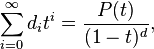
where d is the dimension of the ideal and $P(t)$ is a polynomial such that $P(1)$ is the degree of the ideal.

Although the dimension and the degree do not depend on the choice of the monomial ordering, the Hilbert series and the polynomial $P(t)$ change when one changes of monomial ordering.

Most computer algebra systems that provide functions to compute Gröbner bases provide also functions for computing the Hilbert series, and thus also the dimension and the degree.

Elimination

The computation of Gröbner bases for an elimination monomial ordering allows computational elimination theory. This is based on the following theorem.

Let us consider a polynomial ring $K[x_{1},\ldots ,x_{n},y_{1},\ldots ,y_{m}]=K[X,Y],$ in which the variables are split into two subsets X and Y. Let us also choose an elimination monomial ordering "eliminating" X, that is a monomial ordering for which two monomials are compared by comparing first the X-parts, and, in case of equality only, considering the Y-parts. This implies that a monomial containing an X-variable is greater than every monomial independent of X. If G is a Gröbner basis of an ideal I for this monomial ordering, then $G\cap K[Y]$ is a Gröbner basis of $I\cap K[Y]$ (this ideal is often called the elimination ideal). Moreover, a polynomial belongs to $G\cap K[Y]$ if and only if its leading term belongs to $G\cap K[Y]$ (this makes very easy the computation of $G\cap K[Y]$ , as only the leading monomials need to be checked).

This elimination property has many applications, some of them are reported in the next sections.

Another application, in algebraic geometry, is that elimination realizes the geometric operation of projection of an affine algebraic set into a subspace of the ambient space: with above notation, the (Zariski closure of) the projection of the algebraic set defined by the ideal I into the Y-subspace is defined by the ideal $I\cap K[Y].$

The lexicographical ordering such that $x_{1}>\cdots >x_{n}$ is an elimination ordering for every partition $\{x_{1},\ldots ,x_{k}\},\{x_{{k+1}},\ldots ,x_{n}\}.$ Thus a Gröbner basis for this ordering carries much more information than usually necessary. This may explain why Gröbner bases for the lexicographical ordering are usually the most difficult to compute.

Intersecting ideals

If I and J are two ideals generated respectively by {f₁, ..., f_m} and {g₁, ..., g_k}, then a single Gröbner basis computation produces a Gröbner basis of their intersection I ∩ J. For this, one introduces a new indeterminate t, and one uses an elimination ordering such that the first block contains only t and the other block contains all the other variables (this means that a monomial containing t is greater than every monomial that do not contain t. With this monomial ordering, a Gröbner basis of I ∩ J consists in the polynomials that do not contain t, in the Gröbner basis of the ideal

$K=\langle t^{2},tf_{1},\ldots ,tf_{m},(1-t)g_{1},\ldots ,(1-t)g_{k}\rangle .$

In other words, I ∩ J is obtained by eliminating t in K. This may be proven by remarking that the ideal K consists in the polynomials $(a-b)t+b$ such that $a\in I$ and $b\in J$ . Such a polynomial is independent fo t if and only a=b, which means that $b\in I\cap J.$

Implicitization of a rational curve

A rational curve is an algebraic curve that has a parametric equation of the form

${\begin{aligned}x_{1}&={\frac {f_{1}(t)}{g_{1}(t)}}\\\vdots \\x_{n}&={\frac {f_{n}(t)}{g_{n}(t)}},\end{aligned}}$

where $f_{i}(t)$ and $g_{i}(t)$ are univariate polynomials for 1 ≤ i ≤ n. One may (and will) suppose that $f_{i}(t)$ and $g_{i}(t)$ are coprime (they have no non-constant common factors).

Implicitization consists in computing the implicit equations of such a curve. In case of n = 2, that is for plane curves, this may be computed with the resultant. The implicit equation is the following resultant:

${\text{Res}}_{t}(g_{1}x_{1}-f_{1},g_{2}x_{2}-f_{2}).$

Elimination with Gröbner bases allow to implicitize for any value of n, simply by eliminating t in the ideal $\langle g_{1}x_{1}-f_{1},\ldots ,g_{n}x_{2}-f_{n}\rangle .$ If n = 2, the result is the same as with the resultant, if the map $t\mapsto (x_{1},x_{2})$ is injective for almost every t. In the other case, the resultant is a power of the result of the elimination.

Saturation

When modeling a problem by polynomial equations, it is highly frequent that some quantities are supposed to be non zero, because, if they are zero, the problem becomes very different. For example, when dealing with triangles, many properties become false if the triangle is degenerated, that is if the length of one side is equal to the sum of the lengths of the other sides. In such situations, there is no hope to deduce relevant information from the polynomial system if the degenerate solutions are not dropped out. More precisely, the system of equations defines an algebraic set which may have several irreducible components, and one has to remove the components on which the degeneracy conditions are everywhere zero.

This is done by saturating the equations by the degeneracy conditions, which may be done by using the elimination property of Gröbner bases.

Definition of the saturation

The localization of a ring consists in adjoining to it the formal inverses of some elements. This section concerns only the case of a single element, or equivalently a finite number of elements (adjoining the inverses of several elements is equivalent to adjoin the inverse of their product. The localization of a ring R by an element f is the ring $R_{f}=R[t]/(1-ft),$ where t is a new indeterminate representing the inverse of f. The localization of an ideal I of R is the ideal $R_{f}I$ of $R_{f}.$ When R is a polynomial ring, computing in $R_{f}$ is not efficient, because of the need to manage the denominators. Therefore, the operation of localization is usually replaced by the operation of saturation.

The saturation with respect to f of an ideal I in R is the inverse image of $R_{f}I$ under the canonical map from R to $R_{f}.$ It is the ideal $I:f^{\infty }=\{g\in R|(\exists k\in {\mathbb N})f^{n}g\in I\}$ consisting in all elements of R whose products by some power of f belongs to I.

If J is the ideal generated by I and 1-ft in R[t], then $I:f^{\infty }=J\cap R.$ It follows that, if R is a polynomial ring, a Gröbner basis computation eliminating t allows to compute a Gröbner basis of the saturation of an ideal by a polynomial.

The important property of the saturation, which ensures that it removes from the algebraic set defined by the ideal I the irreducible components on which the polynomial f is zero is the following: The primary decomposition of $I:f^{\infty }$ consists in the components of the primary decomposition of I that do not contain any power of f.

Computation of the saturation

A Gröbner basis of the saturation by f of a polynomial ideal generated by a finite set of polynomials F, may be obtained by eliminating t in $F\cup \{1-tf\},$ that is by keeping the polynomials independent of t in the Gröbner basis of $F\cup \{1-tf\}$ for an elimination ordering eliminating t.

Instead of using F, one may also start from a Gröbner basis of F. It depends on the problems, which method is most efficient. However, if the saturation does not remove any component, that is if the ideal is equal to its saturated ideal, computing first the Gröbner basis of F is usually faster. On the other hand if the saturation removes some components, the direct computation may be dramatically faster.

If one want to saturate with respect to several polynomials $f_{1},\ldots ,f_{k}$ or with respect to a single polynomial which is a product $f=f_{1}\ldots f_{k},$ there are three ways to proceed, that give the same result but may have very different computation times (it depends on the problem which is the most efficient).

Saturating by $f=f_{1}\ldots f_{k}$ in a single Gröbner basis computation.
Saturating by $f_{1},$ then saturating the result by $f_{2},$ and so on.
Adding to F or to its Gröbner basis the polynomials $1-t_{1}f_{1},\ldots ,1-t_{k}f_{k},$ and eliminating the $t_{i}$ in a single Gröbner basis computation.

Effective Nullstellensatz

Hilbert's Nullstellensatz has two versions. The first one asserts that a set of polynomials has an empty set of common zeros in an algebraic closure of the field of the coefficients if and only if 1 belongs to the generated ideal. This is easily tested with a Gröbner basis computation, because 1 belongs to an ideal if and only if 1 belongs to the Gröbner basis of the ideal, for any monomial ordering.

The second version asserts that the set of common zeros (in an algebraic closure of the field of the coefficients) of an ideal is contained in the hypersurface of the zeros of a polynomial f, if and only if a power of f belongs to the ideal. This may be tested by a saturating the ideal by f; in fact, a power of f belongs to the ideal if and only if the saturation by f provides a Gröbner basis containing 1.

Implicitization in higher dimension

By definition, an affine rational variety of dimension k may be described by parametric equations of the form

${\begin{aligned}x_{1}&={\frac {p_{1}}{p_{0}}}\\\vdots \\x_{n}&={\frac {p_{n}}{p_{0}}},\end{aligned}}$

where $p_{0},\ldots ,p_{n}$ are n+1 polynomials in the k variables (parameters of the parameterization) $t_{1},\ldots ,t_{k}.$ Thus the parameters $t_{1},\ldots ,t_{k}$ and the coordinates $x_{1},\ldots ,x_{n}$ of the points of the variety are zeros of the ideal

$I=\left\langle p_{0}x_{1}-p_{1},\ldots ,p_{0}x_{n}-p_{n}\right\rangle .$

One could guess that it suffices to eliminate the parameters to obtain the implicit equations of the variety, as it has been done in the case of curves. Unfortunately this is not always the case. If the $p_{i}$ have a common zero (sometimes called base point), every irreducible component of the non-empty algebraic set defined by the $p_{i}$ is an irreducible component of the algebraic set defined by I. It follows that, in this case, the direct elimination of the $t_{i}$ provides an empty set of polynomials.

Therefore, if k>1, two Gröbner basis computations are needed to implicitize:

Saturate $I$ by $p_{0}$ to get a Gröbner basis $G$
Eliminate the $t_{i}$ from $G$ to get a Gröbner basis of the ideal (of the implicit equations) of the variety.

References

↑ Lazard, D. (1983). "Gröbner bases, Gaussian elimination and resolution of systems of algebraic equations". Computer Algebra. Lecture Notes in Computer Science 162. pp. 146–156. doi:10.1007/3-540-12868-9_99. ISBN 978-3-540-12868-7.
↑ Vladimir P. Gerdt, Yuri A. Blinkov (1998). Involutive Bases of Polynomial Ideals, Mathematics and Computers in Simulation, 45:519ff
↑ David Cox, John Little, and Donal O'Shea (1997). Ideals, Varieties, and Algorithms: An Introduction to Computational Algebraic Geometry and Commutative Algebra. Springer. ISBN 0-387-94680-2.
↑ Allan Steel's Gröbner Basis Timings Page

External links

Faugère's own implementation of his F4 algorithm
Hazewinkel, Michiel, ed. (2001), "Gröbner basis", Encyclopedia of Mathematics, Springer, ISBN 978-1-55608-010-4
B. Buchberger, Groebner Bases: A Short Introduction for Systems Theorists in Proceedings of EUROCAST 2001.
Buchberger, B. and Zapletal, A. Gröbner Bases Bibliography.
Comparative Timings Page for Gröbner Bases Software
Prof. Bruno Buchberger Bruno Buchberger
Weisstein, Eric W., "Gröbner Basis", MathWorld.
Gröbner basis introduction on Scholarpedia

This article is issued from Wikipedia. The text is available under the Creative Commons Attribution/Share Alike; additional terms may apply for the media files.