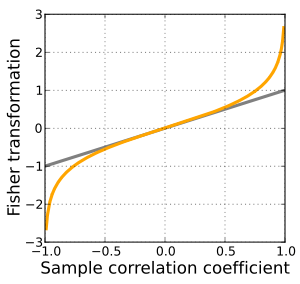
Fisher transformation

From Wikipedia, the free encyclopedia

"Fisher z-transformation" redirects here. It is not to be confused with Fisher's z-distribution.

For standard z-score in statistics, see Standard score. For z-transformation to complex number domain, see Z-transform.

A graph of the transformation. The untransformed sample correlation coefficient is plotted on the horizontal axis, and the transformed coefficient is plotted on the vertical axis. The identity function is also shown for comparison.

In statistics, hypotheses about the value of the population correlation coefficient ρ between variables X and Y can be tested using the Fisher transformation^[1]^[2] (aka Fisher z-transformation) applied to the sample correlation coefficient r.

Definition

The transformation is defined by:

$z={1 \over 2}\ln \left({1+r \over 1-r}\right)=\operatorname {arctanh}(r),$

where "ln" is the natural logarithm function and "arctanh" is the inverse hyperbolic function.

If (X, Y) has a bivariate normal distribution, and if the (X_i, Y_i) pairs used to form r are independent for i = 1, ..., n, then z is approximately normally distributed with mean

${1 \over 2}\ln \left({{1+\rho } \over {1-\rho }}\right),$

and standard error

${1 \over {\sqrt {N-3}}},$

where N is the sample size.

This transformation, and its inverse

$r={{\exp(2z)-1} \over {\exp(2z)+1}}=\operatorname {tanh}(z),$

can be used to construct a confidence interval for ρ.

Discussion

The Fisher transformation is an approximate variance-stabilizing transformation for r when X and Y follow a bivariate normal distribution. This means that the variance of z is approximately constant for all values of the population correlation coefficient ρ. Without the Fisher transformation, the variance of r grows smaller as |ρ| gets closer to 1. Since the Fisher transformation is approximately the identity function when |r| < 1/2, it is sometimes useful to remember that the variance of r is well approximated by 1/N as long as |ρ| is not too large and N is not too small. This is related to the fact that the asymptotic variance of r is 1 for bivariate normal data.

The behavior of this transform has been extensively studied since Fisher introduced it in 1915. Fisher himself found the exact distribution of z for data from a bivariate normal distribution in 1921; Gayen, 1951^[3] determined the exact distribution of z for data from a bivariate Type A Edgeworth distribution. Hotelling in 1953 calculated the Taylor series expressions for the moments of z and several related statistics^[4] and Hawkins in 1989 discovered the asymptotic distribution of z for data from a distribution with bounded fourth moments.^[5]

Other uses

While the Fisher transformation is mainly associated with the Pearson product-moment correlation coefficient for bivariate normal observations, it can also be applied to Spearman's rank correlation coefficient in more general cases. A similar result for the asymptotic distribution applies, but with a minor adjustment factor: see the latter article for details.

References

↑ Fisher, R.A. (1915). "Frequency distribution of the values of the correlation coefficient in samples of an indefinitely large population". Biometrika (Biometrika Trust) 10 (4): 507–521. JSTOR 2331838.
↑ Fisher, R.A. (1921). "On the `probable error' of a coefficient of correlation deduced from a small sample". Metron 1: 3–32.
↑ Gayen, A.K. (1951). "The Frequency Distribution of the Product-Moment Correlation Coefficient in Random Samples of Any Size Drawn from Non-Normal Universes". Biometrika (Biometrika Trust) 38 (1/2): 219–247. JSTOR 2332329.
↑ Hotelling, H (1953). "New light on the correlation coefficient and its transforms". Journal of the Royal Statistical Society, Series B (Blackwell Publishing) 15 (2): 193–225. JSTOR 2983768.
↑ Hawkins, D.L. (1989). "Using U statistics to derive the asymptotic distribution of Fisher's Z statistic". The American Statistician (American Statistical Association) 43 (4): 235–237. doi:10.2307/2685369. JSTOR 2685369.

Statistics

Descriptive statistics

Continuous data

Location	Mean (Arithmetic, Geometric, Harmonic) Median Mode

Dispersion	Range Standard deviation Coefficient of variation Percentile Interquartile range

Shape	Variance Skewness Kurtosis Moments L-moments

Count data

Index of dispersion

Summary tables

Dependence

Statistical graphics

Data collection

Designing studies	Effect size Standard error Statistical power Sample size determination

Survey methodology	Sampling Stratified sampling Cluster sampling Opinion poll Questionnaire

Controlled experiment	Design of experiments Randomized experiment Random assignment Replication Blocking Factorial experiment Optimal design

Uncontrolled studies	Natural experiment Quasi-experiment Observational study

Statistical inference

Statistical theory	Sampling distribution Order statistic Scan statistic Record value Sufficiency Completeness Exponential family Permutation test (Randomization test) Empirical distribution Bootstrap U statistic Efficiency Asymptotics Robustness

Frequentist inference	Unbiased estimator (Mean unbiased minimum variance, Median unbiased) Biased estimators (Maximum likelihood, Method of moments, Minimum distance, Density estimation) Confidence interval Testing hypotheses Power Parametric tests (Likelihood-ratio, Wald, Score)

Specific tests	Z (normal) Student's t-test F Goodness of fit (Chi-squared, G, Sample source, sample normality, Skewness & kurtosis Normality, Model comparison, Model quality) Signed-rank (1-sample, 2-sample, 1-way anova) Shapiro–Wilk Kolmogorov–Smirnov

Bayesian inference	Bayesian probability Prior Posterior Credible interval Bayes factor Bayesian estimator Maximum posterior estimator

Correlation and regression analysis

Correlation	Pearson product–moment correlation Partial correlation Confounding variable Coefficient of determination

Regression analysis	Errors and residuals Regression model validation Mixed effects models Simultaneous equations models MARS

Linear regression	Simple linear regression Ordinary least squares General linear model Bayesian regression

Non-standard predictors	Nonlinear regression Nonparametric Semiparametric Isotonic Robust Heteroscedasticity Homoscedasticity

Generalized linear model	Exponential families Logistic (Bernoulli) Binomial Poisson

Partition of variance	Analysis of variance (ANOVA) Analysis of covariance Multivariate ANOVA Degrees of freedom

Categorical, multivariate, time-series, or survival analysis

Categorical data

Multivariate statistics

Time series analysis

General	Decomposition Trend Stationarity Seasonal adjustment Exponential smoothing Cointegration

Specific tests	Granger causality Q-Statistic Durbin–Watson

Time domain	ACF PACF XCF ARMA model ARIMA model ARCH Vector autoregression

Frequency domain	Spectral density estimation Fourier analysis

Survival analysis

Applications

Biostatistics	Bioinformatics Clinical trials & studies Epidemiology Medical statistics

Engineering statistics	Chemometrics Methods engineering Probabilistic design Process & Quality control Reliability System identification

Social statistics	Actuarial science Census Crime statistics Demography Econometrics National accounts Official statistics Population Psychometrics

Spatial statistics	Cartography Environmental statistics Geographic information system Geostatistics Kriging

Category
Portal
Outline
Index

This article is issued from Wikipedia. The text is available under the Creative Commons Attribution/Share Alike; additional terms may apply for the media files.