Elastic map
Elastic maps provide a tool for nonlinear dimensionality reduction. By their construction, they are system of elastic springs embedded in the data space.[1] This system approximates a low-dimensional manifold. The elastic coefficients of this system allow the switch from completely unstructured k-means clustering (zero elasticity) to the estimators located closely to linear PCA manifolds (for high bending and low stretching modules). With some intermediate values of the elasticity coefficients, this system effectively approximates non-linear principal manifolds. This approach is based on a mechanical analogy between principal manifolds, that are passing through "the middle" of data distribution, and elastic membranes and plates. The method was developed by A.N. Gorban, A.Y. Zinovyev and A.A. Pitenko in 1996–1998.
Energy of elastic map
Let data set be a set of vectors  in a finite-dimensional Euclidean space. The elastic map is represented by a set of nodes
  in the same space. Each datapoint
  has a host node, namely the closest node (if there are several closest nodes then one takes the node with the smallest number). The data set is divided on classes
  .
.
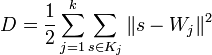
The approximation energy D is the distortion
-
 ,
,
this is the energy of the springs with unit elasticity which connect each data point with its host node. It is possible to apply weighting factors to the terms of this sum, for example to reflect the standard deviation of the probability density function of any subset of data points  .
.
On the set of nodes an additional structure is defined. Some pairs of nodes,  , are connected by elastic edges. Call this set of pairs
  . Some triplets of nodes,
  , form bending ribs. Call this set of triplets
  .
.
- The stretching energy is
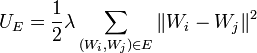 ,
, - The bending energy is
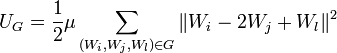 ,
,
where  and
and  are the stretching and bending moduli respectively. The stretching energy is sometimes referred to as the "membrane" term, while the bending energy is referred to as the "thin plate" term.[6]
For example, on the 2D rectangular grid the elastic edges are just vertical and horizontal edges (pairs of closest vertices) and the bending ribs are the vertical or horizontal triplets of consecutive (closest) vertices.
- The total energy of the elastic map is thus

The position of the nodes  is determined by the mechanical equilibrium of the elastic map, i.e. its location is such that it minimizes the total energy
  .
.
Expectation-maximization algorithm
For a given splitting of the dataset in classes  minimization of the quadratic functional is a linear problem with the sparse matrix of coefficients. Therefore, similarly to PCA or k-means, a splitting method is used:
- For given find
 ;
; - For given minimize and find ;
- If no change, terminate.
This expectation-maximization algorithm guarantees a local minimum of . For improving the approximation various additional methods are proposed. For example, the softening strategy is used. This strategy
starts with a rigid grids (small length, small bending and large elasticity modules
and coefficients) and finishes with soft grids (small and ). The training goes in several epochs, each epoch with its own grid rigidness. Another adaptive strategy is growing net: one starts from small amount of nodes and gradually adds new nodes. Each epoch goes with its own number of nodes.
Applications
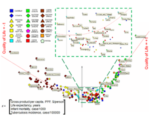
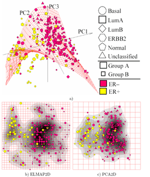
Most important applications are in bioinformatics[7] ,[8] for exploratory data analysis and visualisation of multidimensional data, for data visualisation in economics, social and political sciences,[9] as an auxiliary tool for data mapping in geographic informational systems and for visualisation of data of various nature.
Recently, the method is adapted as a support tool in the decision process underlying the selection, optimization, and management of financial portfolios.[10]
References
- ↑ 1.0 1.1 A. N. Gorban, A. Y. Zinovyev, Principal Graphs and Manifolds, In: Handbook of Research on Machine Learning Applications and Trends: Algorithms, Methods and Techniques, Olivas E.S. et al Eds. Information Science Reference, IGI Global: Hershey, PA, USA, 2009. 28–59.
- ↑ Wang, Y., Klijn, J.G., Zhang, Y., Sieuwerts, A.M., Look, M.P., Yang, F., Talantov, D., Timmermans, M., Meijer-van Gelder, M.E., Yu, J. et al.: Gene expression profiles to predict distant metastasis of lymph-node-negative primary breast cancer. Lancet 365, 671–679 (2005); Data online
- ↑ A. Zinovyev, ViDaExpert - Multidimensional Data Visualization Tool (free for non-commercial use). Institut Curie, Paris.
- ↑ A. Zinovyev, ViDaExpert overview, IHES (Institut des Hautes Études Scientifiques), Bures-Sur-Yvette, Île-de-France.
- ↑ A. N. Gorban, A. Zinovyev, Principal manifolds and graphs in practice: from molecular biology to dynamical systems, International Journal of Neural Systems, Vol. 20, No. 3 (2010) 219–232.
- ↑ Michael Kass, Andrew Witkin, Demetri Terzopoulos, Snakes: Active contour models, Int.J. Computer Vision, 1988 vol 1-4 pp.321-331
- ↑ A.N. Gorban, B. Kegl, D. Wunsch, A. Zinovyev (Eds.), Principal Manifolds for Data Visualisation and Dimension Reduction, LNCSE 58, Springer: Berlin – Heidelberg – New York, 2007. ISBN 978-3-540-73749-0
- ↑ M. Chacón, M. Lévano, H. Allende, H. Nowak, Detection of Gene Expressions in Microarrays by Applying Iteratively Elastic Neural Net, In: B. Beliczynski et al. (Eds.), Lecture Notes in Computer Sciences, Vol. 4432, Springer: Berlin – Heidelberg 2007, 355–363.
- ↑ A. Zinovyev, Data visualization in political and social sciences, In: SAGE "International Encyclopedia of Political Science", Badie, B., Berg-Schlosser, D., Morlino, L. A. (Eds.), 2011.
- ↑ M. Resta, Portfolio optimization through elastic maps: Some evidence from the Italian stock exchange, Knowledge-Based Intelligent Information and Engineering Systems, B. Apolloni, R.J. Howlett and L. Jain (eds.), Lecture Notes in Computer Science, Vol. 4693, Springer: Berlin – Heidelberg, 2010, 635-641.