Adaptive mesh refinement
- This article is about the use of adaptive meshing in numerical analysis. See Subdivision surface for the use of adaptive techniques in Computer Graphics modelling.
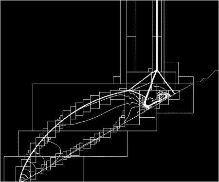
In numerical analysis, adaptive mesh refinement is a method of changing the accuracy of a solution in certain regions, during the time the solution is being calculated. When solutions are calculated numerically, they are often constrained to discrete locations which constitute the computational grid, or 'mesh'. For example, when calculating a solution to the shallow water equations, the solution (water height) might only be calculated for points every few feet apart - and one would assume that in between those points the height varies smoothly. The limiting factor to the resolution of the solution is thus the grid spacing: there will be no features of the numerical solution on scales smaller than the grid-spacing. Adaptive mesh refinement (AMR) changes the spacing of grid points, to change how accurately the solution is known in that region. In the shallow water example, the grid might in general be spaced every few feet - but it could be adaptively refined to have grid points every few inches in places where there are large waves.
If the region in which higher resolution is desired remains localized over the course of the computation, then static mesh refinement can be used - in which the grid is more finely spaced in some regions than others, but maintains its shape over time.
The advantages of a dynamic gridding scheme are:
- Increased computational savings over a static grid approach.
- Increased storage savings over a static grid approach.
- Complete control of grid resolution, compared to the fixed resolution of a static grid approach, or the Lagrangian-based adaptivity of smoothed particle hydrodynamics.
Introduction to adaptive mesh refinement

In a series of papers, Marsha Berger, Joseph Oliger, and Phillip Colella developed an algorithm for dynamic griding called local adaptive mesh refinement. The algorithm begins with the entire computational domain covered with a coarsely resolved base-level regular Cartesian grid. As the calculation progresses, individual grid cells are tagged for refinement, using a criterion that can either be user-supplied (for example mass per cell remains constant, hence higher density regions are more highly resolved) or based on Richardson extrapolation.
All tagged cells are then refined, meaning that a finer grid is overlaid on the coarse one. After refinement, individual grid patches on a single fixed level of refinement are passed off to an integrator which advances those cells in time. Finally, a correction procedure is implemented to correct the transfer along coarse-fine grid interfaces, to ensure that the amount of any conserved quantity leaving one cell exactly balances the amount entering the bordering cell. If at some point the level of refinement in a cell is greater than required, the high resolution grid may be removed and replaced with a coarser grid.
This allows the user to solve problems that are completely intractable on a uniform grid; for example, astrophysicists have used AMR to model a collapsing giant molecular cloud core down to an effective resolution of 131,072 cells per initial cloud radius, corresponding to a resolution of 1015 cells on a uniform grid.[1]
Advanced mesh refinement has been introduced via functionals.[2] Functionals allow the ability to generate grids and provide mesh adaptation. Some advanced functionals include the Winslow and modified Liao functionals.[3]
References
- Berger, M. J.; Colella, P. (1989). "Local adaptive mesh refinement for shock hydrodynamics". J. Comput. Phys. (Elsevier) 82: 64–84.
- ↑ Klein, Richard (1999). "Star formation with 3-D adaptive mesh refinement: the collapse and fragmentation of molecular clouds". Journal of Computational and Applied Mathematics 109 (1-2): 123–152. doi:10.1016/S0377-0427(99)00156-9. Retrieved February 16, 2011.
- ↑ Huang, Weizhang; Russell, Robert D. "Adaptive Moving Mesh Methods".
- ↑ Khattri, Sanjay Kumar. "Grid Generation and Adaptation by Functionals".