Toeplitz matrix
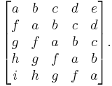
In linear algebra, a Toeplitz matrix or diagonal-constant matrix, named after Otto Toeplitz, is a matrix in which each descending diagonal from left to right is constant. For instance, the following matrix is a Toeplitz matrix:
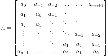
Any n×n matrix A of the form
is a Toeplitz matrix. If the i,j element of A is denoted Ai,j, then we have
Contents |
Solving a Toeplitz system
A matrix equation of the form
is called a Toeplitz system if A is a Toeplitz matrix. If A is an  Toeplitz matrix, then the system has only 2n−1 degrees of freedom, rather than n2. We might therefore expect that the solution of a Toeplitz system would be easier, and indeed that is the case.
Toeplitz systems can be solved by the Levinson algorithm in Θ(n2) time.[1] Variants of this algorithm have been shown to be weakly stable (i.e. they exhibit numerical stability for well-conditioned linear systems).[2] The algorithm can also be used to find the determinant of a Toeplitz matrix in O(n2) time.[3]
A Toeplitz matrix can also be decomposed (i.e. factored) in O(n2) time.[4] The Bareiss algorithm for an LU decomposition is stable.[5] An LU decomposition gives a quick method for solving a Toeplitz system, and also for computing the determinant.
Algorithms that are asymptotically faster than those of Bareiss and Levinson have been described in the literature.[6][7][8][9]
General properties
A Toeplitz matrix may be defined as a matrix A where Ai,j = ci−j, for constants c1−n … cn−1.
Two Toeplitz matrices may be added in O(n) time and multiplied in O(n2).
Toeplitz matrices are persymmetric. Symmetric Toeplitz matrices are both centrosymmetric and bisymmetric.
Toeplitz matrices are also closely connected with Fourier series, because the multiplication operator by a trigonometric polynomial, compressed to a finite-dimensional space, can be represented by such a matrix.
All Toeplitz matrices commute asymptotically. This means they diagonalize in the same basis when the row and column dimension tends to infinity.
Discrete convolution
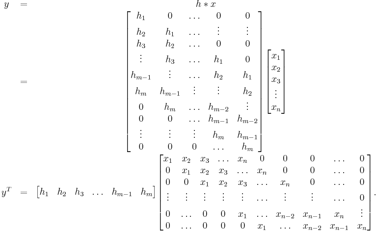
The convolution operation can be constructed as a matrix multiplication, where one of the inputs is converted into a Toeplitz matrix. For example, the convolution of  and
and  can be formulated as:

This approach can be extended to compute autocorrelation, cross-correlation, moving average etc.
See also
- Circulant matrix, a Toeplitz matrix with the additional property that
 .
. - Hankel matrix, a Toeplitz matrix "upside down".
- Toeplitz operator, a Toeplitz matrix with infinitely many rows and columns.
Notes
References
- A.W. Bojanczyk, R.P. Brent, F.R. De Hoog, D.R. Sweet (1995), "On the stability of the Bareiss and related Toeplitz factorization algorithms", SIAM Journal on Matrix Analysis and Applications, 16: 40-57.
- Brent R.P. (1999), "Stability of fast algorithms for structured linear systems", Fast Reliable Algorithms for Matrices with Structure (editors—T. Kailath, A.H. Sayed), ch.4 (SIAM).
- Chan R.H.-F., Jin X.-Q. (2007), An Introduction to Iterative Toeplitz Solvers (SIAM).
- Chandrasekeran S., Gu M., Sun X., Xia J., Zhu J. (2007), "A superfast algorithm for Toeplitz systems of linear equations", SIAM Journal on Matrix Analysis and Applications, 29: 1247-1266. doi:10.1137/040617200
- Chen W.W., Hurvich C.M., Lu Y. (2006), "On the correlation matrix of the discrete Fourier transform and the fast solution of large Toeplitz systems for long-memory time series", Journal of the American Statistical Association, 101: 812-822. doi:10.1198/016214505000001069
- Golub G.H., van Loan C.F. (1996), Matrix Computations (Johns Hopkins University Press), Section 4.7—Toeplitz and Related Systems.
- Gray R.M., Toeplitz and Circulant Matrices: A Review (Now Publishers).
- Krishna, H.; Wang, Y. (1993). "The Split Levinson Algorithm is weakly stable". SIAM Journal on Numerical Analysis 30 (5): 1498–1508. doi:10.1137/0730078. http://scitation.aip.org/getabs/servlet/GetabsServlet?prog=normal&id=SJNAAM000030000005001498000001&idtype=cvips&gifs=yes.
- Monahan J.F. (2011), Numerical Methods of Statistics (Cambridge University Press), §4.5—Toeplitz systems.
- Press W.H., Teukolsky S.A., Vetterling W.T., Flannery B.P. (2007), Numerical Recipes: The Art of Scientific Computing, Third edition (Cambridge University Press), §2.8.2—Toeplitz matrices. ISBN 978-0-521-88068-8
- Stewart M. (2003), "A superfast Toeplitz solver with improved numerical stability", SIAM Journal on Matrix Analysis and Applications, 25: 669-693. doi:10.1137/S089547980241791X


