Support vector machine

A support vector machine (SVM) is a concept in statistics and computer science for a set of related supervised learning methods that analyze data and recognize patterns, used for classification and regression analysis. The standard SVM takes a set of input data and predicts, for each given input, which of two possible classes forms the input, making the SVM a non-probabilistic binary linear classifier. Given a set of training examples, each marked as belonging to one of two categories, an SVM training algorithm builds a model that assigns new examples into one category or the other. An SVM model is a representation of the examples as points in space, mapped so that the examples of the separate categories are divided by a clear gap that is as wide as possible. New examples are then mapped into that same space and predicted to belong to a category based on which side of the gap they fall on.

Formal definition

More formally, a support vector machine constructs a hyperplane or set of hyperplanes in a high- or infinite- dimensional space, which can be used for classification, regression, or other tasks. Intuitively, a good separation is achieved by the hyperplane that has the largest distance to the nearest training data points of any class (so-called functional margin), since in general the larger the margin the lower the generalization error of the classifier.

Whereas the original problem may be stated in a finite dimensional space, it often happens that the sets to discriminate are not linearly separable in that space. For this reason, it was proposed that the original finite-dimensional space be mapped into a much higher-dimensional space, presumably making the separation easier in that space. To keep the computational load reasonable, the mapping used by SVM schemes are designed to ensure that dot products may be computed easily in terms of the variables in the original space, by defining them in terms of a kernel function $K(x,y)$ selected to suit the problem.^[1] The hyperplanes in the higher dimensional space are defined as the set of points whose inner product with a vector in that space is constant. The vectors defining the hyperplanes can be chosen to be linear combinations with parameters $\alpha_i$ of images of feature vectors that occur in the data base. With this choice of a hyperplane, the points x in the feature space that are mapped into the hyperplane are defined by the relation: 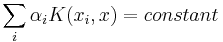$\sum_i{ \alpha_i K(x_i,x)} = constant$ Note that if $K(x,y)$ becomes small as $y$ grows further from $x$ , each element in the sum measures the degree of closeness of the test point $x$ to the corresponding data base point $x_i$ . In this way, the sum of kernels above can be used to measure the relative nearness of each test point to the data points originating in one or the other of the sets to be discriminated. Note the fact that the set of points $x$ mapped into any hyperplane can be quite convoluted as a result allowing much more complex discrimination between sets which are not convex at all in the original space.

History

The original SVM algorithm was invented by Vladimir Vapnik and the current standard incarnation (soft margin) was proposed by Vapnik and Corinna Cortes in 1995.^[2]

Motivation

Classifying data is a common task in machine learning. Suppose some given data points each belong to one of two classes, and the goal is to decide which class a new data point will be in. In the case of support vector machines, a data point is viewed as a p-dimensional vector (a list of p numbers), and we want to know whether we can separate such points with a (p − 1)-dimensional hyperplane. This is called a linear classifier. There are many hyperplanes that might classify the data. One reasonable choice as the best hyperplane is the one that represents the largest separation, or margin, between the two classes. So we choose the hyperplane so that the distance from it to the nearest data point on each side is maximized. If such a hyperplane exists, it is known as the maximum-margin hyperplane and the linear classifier it defines is known as a maximum margin classifier; or equivalently, the perceptron of optimal stability.

Linear SVM

We are given some training data $\mathcal{D}$ , a set of n points of the form

$\mathcal{D} = \left\{ (\mathbf{x}_i, y_i)\mid\mathbf{x}_i \in \mathbb{R}^p,\, y_i \in \{-1,1\}\right\}_{i=1}^n$

where the y_i is either 1 or −1, indicating the class to which the point $\mathbf{x}_i$ belongs. Each $\mathbf{x}_i$ is a p-dimensional real vector. We want to find the maximum-margin hyperplane that divides the points having $y_i=1$ from those having $y_i=-1$ . Any hyperplane can be written as the set of points $\mathbf{x}$ satisfying

$\mathbf{w}\cdot\mathbf{x} - b=0,\,$

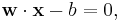
where $\cdot$ denotes the dot product and ${\mathbf{w}}$ the normal vector to the hyperplane. The parameter $\tfrac{b}{\|\mathbf{w}\|}$ determines the offset of the hyperplane from the origin along the normal vector ${\mathbf{w}}$ .

We want to choose the ${\mathbf{w}}$ and $b$ to maximize the margin, or distance between the parallel hyperplanes that are as far apart as possible while still separating the data. These hyperplanes can be described by the equations

$\mathbf{w}\cdot\mathbf{x} - b=1\,$

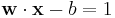
and

$\mathbf{w}\cdot\mathbf{x} - b=-1.\,$

Note that if the training data are linearly separable, we can select the two hyperplanes of the margin in a way that there are no points between them and then try to maximize their distance. By using geometry, we find the distance between these two hyperplanes is $\tfrac{2}{\|\mathbf{w}\|}$ , so we want to minimize $\|\mathbf{w}\|$ . As we also have to prevent data points from falling into the margin, we add the following constraint: for each $i$ either

$\mathbf{w}\cdot\mathbf{x}_i - b \ge 1\qquad\text{ for }\mathbf{x}_i$ of the first class

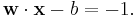
$\mathbf{w}\cdot\mathbf{x}_i - b \le -1\qquad\text{ for }\mathbf{x}_i$ of the second.

This can be rewritten as:

$y_i(\mathbf{w}\cdot\mathbf{x}_i - b) \ge 1, \quad \text{ for all } 1 \le i \le n.\qquad\qquad(1)$

We can put this together to get the optimization problem:

Minimize (in ${\mathbf{w},b}$ )

$\|\mathbf{w}\|$

subject to (for any $i = 1, \dots, n$ )

$y_i(\mathbf{w}\cdot\mathbf{x_i} - b) \ge 1. \,$

Primal form

The optimization problem presented in the preceding section is difficult to solve because it depends on ||w||, the norm of w, which involves a square root. Fortunately it is possible to alter the equation by substituting ||w|| with $\tfrac{1}{2}\|\mathbf{w}\|^2$ (the factor of 1/2 being used for mathematical convenience) without changing the solution (the minimum of the original and the modified equation have the same w and b). This is a quadratic programming optimization problem. More clearly:

Minimize (in ${\mathbf{w},b}$ )

$\frac{1}{2}\|\mathbf{w}\|^2$

subject to (for any $i = 1, \dots, n$ )

$y_i(\mathbf{w}\cdot\mathbf{x_i} - b) \ge 1.$

One could be tempted to express the previous problem by means of non-negative Lagrange multipliers $\alpha_i$ as

$\min_{\mathbf{w},b,\boldsymbol{\alpha}} \left\{ \frac{1}{2}\|\mathbf{w}\|^2 - \sum_{i=1}^{n}{\alpha_i[y_i(\mathbf{w}\cdot \mathbf{x_i} - b)-1]} \right\}$

but this would be wrong. The reason is the following: suppose we can find a family of hyperplanes which divide the points; then all $y_i(\mathbf{w}\cdot\mathbf{x_i} - b) - 1 \ge 0$ . Hence we could find the minimum by sending all $\alpha_i$ to $%2B\infty$ , and this minimum would be reached for all the members of the family, not only for the best one which can be chosen solving the original problem.

Nevertheless the previous constrained problem can be expressed as

$\min_{\mathbf{w},b } \max_{\boldsymbol{\alpha} } \left\{ \frac{1}{2}\|\mathbf{w}\|^2 - \sum_{i=1}^{n}{\alpha_i[y_i(\mathbf{w}\cdot \mathbf{x_i} - b)-1]} \right\}$

that is we look for a saddle point. In doing so all the points which can be separated as $y_i(\mathbf{w}\cdot\mathbf{x_i} - b) - 1 > 0$ do not matter since we must set the corresponding $\alpha_i$ to zero.

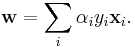
This problem can now be solved by standard quadratic programming techniques and programs. The solution can be expressed by terms of linear combination of the training vectors as

$\mathbf{w} = \sum_{i=1}^n{\alpha_i y_i\mathbf{x_i}}$

Only a few $\alpha_i$ will be greater than zero. The corresponding $\mathbf{x_i}$ are exactly the support vectors, which lie on the margin and satisfy $y_i(\mathbf{w}\cdot\mathbf{x_i} - b) = 1$ . From this one can derive that the support vectors also satisfy

$\mathbf{w}\cdot\mathbf{x_i} - b = 1 / y_i = y_i \iff b = \mathbf{w}\cdot\mathbf{x_i} - y_i$

which allows one to define the offset $b$ . In practice, it is more robust to average over all $N_{SV}$ support vectors:

$b = \frac{1}{N_{SV}} \sum_{i=1}^{N_{SV}}{(\mathbf{w}\cdot\mathbf{x_i} - y_i)}$

Dual form

Writing the classification rule in its unconstrained dual form reveals that the maximum margin hyperplane and therefore the classification task is only a function of the support vectors, the training data that lie on the margin.

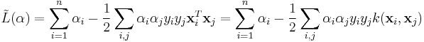
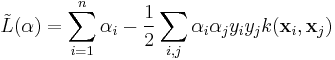
Using the fact, that $\|\mathbf{w}\|^2 = w\cdot w$ and substituting 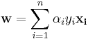$\mathbf{w} = \sum_{i=1}^n{\alpha_i y_i\mathbf{x_i}}$ , one can show that the dual of the SVM reduces to the following optimization problem:

Maximize (in $\alpha_i$ )

$\tilde{L}(\mathbf{\alpha})=\sum_{i=1}^n \alpha_i - \frac{1}{2}\sum_{i, j} \alpha_i \alpha_j y_i y_j \mathbf{x}_i^T \mathbf{x}_j=\sum_{i=1}^n \alpha_i - \frac{1}{2}\sum_{i, j} \alpha_i \alpha_j y_i y_j k(\mathbf{x}_i, \mathbf{x}_j)$

subject to (for any $i = 1, \dots, n$ )

$\alpha_i \geq 0,\,$

and to the constraint from the minimization in $b$

$\sum_{i=1}^n \alpha_i y_i = 0.$

Here the kernel is defined by $k(\mathbf{x}_i,\mathbf{x}_j)=\mathbf{x}_i\cdot\mathbf{x}_j$ .

$W$ can be computed thanks to the $\alpha$ terms:

$\mathbf{w} = \sum_i \alpha_i y_i \mathbf{x}_i.$

Biased and unbiased hyperplanes

For simplicity reasons, sometimes it is required that the hyperplane passes through the origin of the coordinate system. Such hyperplanes are called unbiased, whereas general hyperplanes not necessarily passing through the origin are called biased. An unbiased hyperplane can be enforced by setting $b = 0$ in the primal optimization problem. The corresponding dual is identical to the dual given above without the equality constraint

$\sum_{i=1}^n \alpha_i y_i = 0.$

Soft margin

In 1995, Corinna Cortes and Vladimir Vapnik suggested a modified maximum margin idea that allows for mislabeled examples.^[2] If there exists no hyperplane that can split the "yes" and "no" examples, the Soft Margin method will choose a hyperplane that splits the examples as cleanly as possible, while still maximizing the distance to the nearest cleanly split examples. The method introduces slack variables, $\xi_i$ , which measure the degree of misclassification of the datum $x_i$

$y_i(\mathbf{w}\cdot\mathbf{x_i} - b) \ge 1 - \xi_i \quad 1 \le i \le n. \quad\quad(2)$

The objective function is then increased by a function which penalizes non-zero $\xi_i$ , and the optimization becomes a trade off between a large margin, and a small error penalty. If the penalty function is linear, the optimization problem becomes:

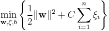
$\min_{\mathbf{w},\mathbf{\xi}, b } \left\{\frac{1}{2} \|\mathbf{w}\|^2 %2B C \sum_{i=1}^n \xi_i \right\}$

subject to (for any $i=1,\dots n$ )

$y_i(\mathbf{w}\cdot\mathbf{x_i} - b) \ge 1 - \xi_i, ~~~~\xi_i \ge 0 .$

This constraint in (2) along with the objective of minimizing $\|\mathbf{w}\|$ can be solved using Lagrange multipliers as done above. One has then to solve the following problem

$\min_{\mathbf{w},\mathbf{\xi}, b } \max_{\boldsymbol{\alpha},\boldsymbol{\beta} } \left \{ \frac{1}{2}\|\mathbf{w}\|^2 %2BC \sum_{i=1}^n \xi_i - \sum_{i=1}^{n}{\alpha_i[y_i(\mathbf{w}\cdot \mathbf{x_i} - b) -1 %2B \xi_i]} - \sum_{i=1}^{n} \beta_i \xi_i \right \}$

with $\alpha_i, \beta_i \ge 0$ .

Dual form

Maximize (in $\alpha_i$ )

$\tilde{L}(\mathbf{\alpha})=\sum_{i=1}^n \alpha_i - \frac{1}{2}\sum_{i, j} \alpha_i \alpha_j y_i y_j k(\mathbf{x}_i, \mathbf{x}_j)$

subject to (for any $i = 1, \dots, n$ )

$0 \leq \alpha_i \leq C,\,$

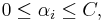
and

$\sum_{i=1}^n \alpha_i y_i = 0.$

The key advantage of a linear penalty function is that the slack variables vanish from the dual problem, with the constant C appearing only as an additional constraint on the Lagrange multipliers. For the above formulation and its huge impact in practice, Cortes and Vapnik received the 2008 ACM Paris Kanellakis Award.^[3] Nonlinear penalty functions have been used, particularly to reduce the effect of outliers on the classifier, but unless care is taken, the problem becomes non-convex, and thus it is considerably more difficult to find a global solution.

Nonlinear classification

The original optimal hyperplane algorithm proposed by Vapnik in 1963 was a linear classifier. However, in 1992, Bernhard Boser, Isabelle Guyon and Vapnik suggested a way to create nonlinear classifiers by applying the kernel trick (originally proposed by Aizerman et al.^[4]) to maximum-margin hyperplanes.^[5] The resulting algorithm is formally similar, except that every dot product is replaced by a nonlinear kernel function. This allows the algorithm to fit the maximum-margin hyperplane in a transformed feature space. The transformation may be nonlinear and the transformed space high dimensional; thus though the classifier is a hyperplane in the high-dimensional feature space, it may be nonlinear in the original input space.

If the kernel used is a Gaussian radial basis function, the corresponding feature space is a Hilbert space of infinite dimensions. Maximum margin classifiers are well regularized, so the infinite dimensions do not spoil the results. Some common kernels include:

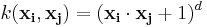
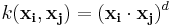
Polynomial (homogeneous): $k(\mathbf{x_i},\mathbf{x_j})=(\mathbf{x_i} \cdot \mathbf{x_j})^d$
Polynomial (inhomogeneous): $k(\mathbf{x_i},\mathbf{x_j})=(\mathbf{x_i} \cdot \mathbf{x_j} %2B 1)^d$
Gaussian radial basis function: 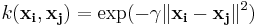$k(\mathbf{x_i},\mathbf{x_j})=\exp(-\gamma \|\mathbf{x_i} - \mathbf{x_j}\|^2)$ , for $\gamma > 0.$ Sometimes parametrized using $\gamma=1/{2 \sigma^2}$
Hyperbolic tangent: 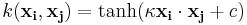$k(\mathbf{x_i},\mathbf{x_j})=\tanh(\kappa \mathbf{x_i} \cdot \mathbf{x_j}%2Bc)$ , for some (not every) $\kappa > 0$ and $c < 0$

The kernel is related to the transform $\varphi(\mathbf{x_i})$ by the equation 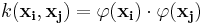$k(\mathbf{x_i}, \mathbf{x_j}) = \varphi(\mathbf{x_i})\cdot \varphi(\mathbf{x_j})$ . The value w is also in the transformed space, with 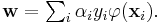$\textstyle\mathbf{w} = \sum_i \alpha_i y_i \varphi(\mathbf{x}_i).$ Dot products with w for classification can again be computed by the kernel trick, i.e. 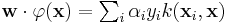$\textstyle \mathbf{w}\cdot\varphi(\mathbf{x}) = \sum_i \alpha_i y_i k(\mathbf{x}_i, \mathbf{x})$ . 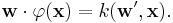However, there does not in general exist a value w' such that $\mathbf{w}\cdot\varphi(\mathbf{x}) = k(\mathbf{w'}, \mathbf{x}).$

Properties

SVMs belong to a family of generalized linear classifiers and can be interpreted as an extension of the perceptron. They can also be considered a special case of Tikhonov regularization. A special property is that they simultaneously minimize the empirical classification error and maximize the geometric margin; hence they are also known as maximum margin classifiers.

A comparison of the SVM to other classifiers has been made by Meyer, Leisch and Hornik.^[6]

Parameter selection

The effectiveness of SVM depends on the selection of kernel, the kernel's parameters, and soft margin parameter C.

A common choice is a Gaussian kernel, which has a single parameter γ. Best combination of C and γ is often selected by a grid-search with exponentially growing sequences of C and γ, for example, $C \in \{ 2^{-5}, 2^{-3}, \dots, 2^{13},2^{15} \}$ ; $\gamma \in \{ 2^{-15},2^{-13}, \dots, 2^{1},2^{3} \}$ . Typically, each combination of parameter choices is checked using cross validation, and the parameters with best cross-validation accuracy are picked. The final model, which is used for testing and for classifying new data, is then trained on the whole training set using the selected parameters.^[7]

Issues

Potential drawbacks of the SVM are the following three aspects:

Uncalibrated class membership probabilities
The SVM is only directly applicable for two-class tasks. Therefore, algorithms that reduce the multi-class task to several binary problems have to be applied; see the multi-class SVM section.
Parameters of a solved model are difficult to interpret.

Extensions

Multiclass SVM

Multiclass SVM aims to assign labels to instances by using support vector machines, where the labels are drawn from a finite set of several elements.

The dominant approach for doing so is to reduce the single multiclass problem into multiple binary classification problems.^[8] Common methods for such reduction include:^[8] ^[9]

Building binary classifiers which distinguish between (i) one of the labels to the rest (one-versus-all) or (ii) between every pair of classes (one-versus-one). Classification of new instances for one-versus-all case is done by a winner-takes-all strategy, in which the classifier with the highest output function assigns the class (it is important that the output functions be calibrated to produce comparable scores). For the one-versus-one approach, classification is done by a max-wins voting strategy, in which every classifier assigns the instance to one of the two classes, then the vote for the assigned class is increased by one vote, and finally the class with most votes determines the instance classification.
DAGSVM^[10]
error-correcting output codes^[11]

Crammer and Singer proposed a multiclass SVM method which casts the multiclass classification problem into a single optimization problem, rather than decomposing it into multiple binary classification problems.^[12]

Transductive support vector machines

Transductive support vector machines extend SVMs in that they could also treat partially labeled data in semi-supervised learning by following the principles of transduction. Here, in addition to the training set $\mathcal{D}$ , the learner is also given a set

$\mathcal{D}^\star = \{ \mathbf{x}^\star_i | \mathbf{x}^\star_i \in \mathbb{R}^p\}_{i=1}^k \,$

of test examples to be classified. Formally, a transductive support vector machine is defined by the following primal optimization problem:^[13]

Minimize (in ${\mathbf{w}, b, \mathbf{y^\star}}$ )

$\frac{1}{2}\|\mathbf{w}\|^2$

subject to (for any $i = 1, \dots, n$ and any $j = 1, \dots, k$ )

$y_i(\mathbf{w}\cdot\mathbf{x_i} - b) \ge 1,\,$

$y^\star_j(\mathbf{w}\cdot\mathbf{x^\star_j} - b) \ge 1,$

and

$y^\star_j \in \{-1, 1\}.\,$

Transductive support vector machines were introduced by Vladimir Vapnik in 1998.

Structured SVM

SVMs have been generalized to structured SVMs, where the label space is structured and of possibly infinite size.

Regression

A version of SVM for regression was proposed in 1996 by Vladimir Vapnik, Harris Drucker, Chris Burges, Linda Kaufman and Alex Smola.^[14] This method is called support vector regression (SVR). The model produced by support vector classification (as described above) depends only on a subset of the training data, because the cost function for building the model does not care about training points that lie beyond the margin. Analogously, the model produced by SVR depends only on a subset of the training data, because the cost function for building the model ignores any training data close to the model prediction (within a threshold $\epsilon$ ). Another SVM version known as least squares support vector machine (LS-SVM) has been proposed in Suykens and Vandewalle.^[15]

Implementation

The parameters of the maximum-margin hyperplane are derived by solving the optimization. There exist several specialized algorithms for quickly solving the QP problem that arises from SVMs, mostly relying on heuristics for breaking the problem down into smaller, more-manageable chunks.

A common method is Platt's Sequential Minimal Optimization (SMO) algorithm, which breaks the problem down into 2-dimensional sub-problems that may be solved analytically, eliminating the need for a numerical optimization algorithm.

Another approach is to use an interior point method that uses Newton-like iterations to find a solution of the Karush–Kuhn–Tucker conditions of the primal and dual problems.^[16] Instead of solving a sequence of broken down problems, this approach directly solves the problem as a whole. To avoid solving a linear system involving the large kernel matrix, a low rank approximation to the matrix is often used in the kernel trick.

References

^ *Press, WH; Teukolsky, SA; Vetterling, WT; Flannery, BP (2007). "Section 16.5. Support Vector Machines". Numerical Recipes: The Art of Scientific Computing (3rd ed.). New York: Cambridge University Press. ISBN 978-0-521-88068-8. http://apps.nrbook.com/empanel/index.html#pg=883.
^ ^a ^b Corinna Cortes and V. Vapnik, "Support-Vector Networks", Machine Learning, 20, 1995. http://www.springerlink.com/content/k238jx04hm87j80g/
^ ACM Website, Press release of March 17th 2009. http://www.acm.org/press-room/news-releases/awards-08-groupa
^ M. Aizerman, E. Braverman, and L. Rozonoer (1964). "Theoretical foundations of the potential function method in pattern recognition learning". Automation and Remote Control 25: 821–837.
^ B. E. Boser, I. M. Guyon, and V. N. Vapnik. A training algorithm for optimal margin classifiers. In D. Haussler, editor, 5th Annual ACM Workshop on COLT, pages 144–152, Pittsburgh, PA, 1992. ACM Press
^ David Meyer, Friedrich Leisch, and Kurt Hornik. The support vector machine under test. Neurocomputing 55(1–2): 169–186, 2003 http://dx.doi.org/10.1016/S0925-2312(03)00431-4
^ Chih-Wei Hsu, Chih-Chung Chang, and Chih-Jen Lin (2003). A Practical Guide to Support Vector Classification (Technical report). Department of Computer Science and Information Engineering, National Taiwan University. http://www.csie.ntu.edu.tw/~cjlin/papers/guide/guide.pdf.
^ ^a ^b Kai-Bo Duan and S. Sathiya Keerthi (2005). "Which Is the Best Multiclass SVM Method? An Empirical Study". Proceedings of the Sixth International Workshop on Multiple Classifier Systems. http://research.yahoo.com/files/multiclass_mcs_kaibo_05.pdf.
^ Chih-Wei Hsu and Chih-Jen Lin (2002). "A Comparison of Methods for Multiclass Support Vector Machines". IEEE Transactions on Neural Networks.
^ Platt, J., Cristianini, N., Shawe-Taylor, J. (2000). "Large margin DAGs for multiclass classification". Advances in Neural Information Processing Systems (MIT Press).
^ Dietterich, T., Bakiri, G. (1995). "Solving Multiclass Learning Problems via Error-Correcting Output Codes". Journal of Artificial Intelligence Research, Vol. 2: 263–286.
^ Koby Crammer and Yoram Singer (2001). "On the Algorithmic Implementation of Multiclass Kernel-based Vector Machines". Journal of Machine Learning Research 2: 265–292.
^ Thorsten Joachims, "Transductive Inference for Text Classification using Support Vector Machines", Proceedings of the 1999 International Conference on Machine Learning (ICML 1999), pp. 200-209.
^ Harris Drucker, Chris J.C. Burges, Linda Kaufman, Alex Smola and Vladimir Vapnik (1997). "Support Vector Regression Machines". Advances in Neural Information Processing Systems 9, NIPS 1996, 155–161, MIT Press.
^ Suykens J.A.K., Vandewalle J., Least squares support vector machine classifiers, Neural Processing Letters, vol. 9, no. 3, Jun. 1999, pp. 293–300.
^ M. Ferris, and T. Munson (2002). "Interior-point methods for massive support vector machines". SIAM Journal on Optimization 13 (3): 783–804. doi:10.1137/S1052623400374379.

External links

A Tutorial on Support Vector Machines for Pattern Recognition by Christopher J. C. Burges. Data Mining and Knowledge Discovery 2:121–167, 1998
www.kernel-machines.org (general information and collection of research papers)
www.support-vector-machines.org (Literature, Review, Software, Links related to Support Vector Machines — Academic Site)
videolectures.net (SVM-related video lectures)
Animation clip: SVM with polynomial kernel visualization.
A very basic SVM tutorial for complete beginners by Tristan Fletcher [1].
www.shogun-toolbox.org (Shogun (toolbox) contains about 20 different implementations of SVMs)
libsvm libsvm is a library of SVMs which is actively patched
liblinear liblinear is a library for large linear classification including some SVMs
flssvm flssvm is a least squares svm implementation written in fortran
Shark Shark is a C++ machine learning library implementing various types of SVMs
dlib dlib is a C++ library for working with kernel methods and SVMs
SVM light is a collection of software tools for learning and classification using SVM.

Bibliography

Sergios Theodoridis and Konstantinos Koutroumbas "Pattern Recognition", 4th Edition, Academic Press, 2009, ISBN 978-1597492720
Nello Cristianini and John Shawe-Taylor. An Introduction to Support Vector Machines and other kernel-based learning methods. Cambridge University Press, 2000. ISBN 0-521-78019-5 ([2] SVM Book)
Huang T.-M., Kecman V., Kopriva I. (2006), Kernel Based Algorithms for Mining Huge Data Sets, Supervised, Semi-supervised, and Unsupervised Learning, Springer-Verlag, Berlin, Heidelberg, 260 pp. 96 illus., Hardcover, ISBN 3-540-31681-7 [3]
Vojislav Kecman: "Learning and Soft Computing — Support Vector Machines, Neural Networks, Fuzzy Logic Systems", The MIT Press, Cambridge, MA, 2001.[4]
Bernhard Schölkopf and A. J. Smola: Learning with Kernels. MIT Press, Cambridge, MA, 2002. (Partly available on line: [5].) ISBN 0-262-19475-9
Bernhard Schölkopf, Christopher J.C. Burges, and Alexander J. Smola (editors). "Advances in Kernel Methods: Support Vector Learning". MIT Press, Cambridge, MA, 1999. ISBN 0-262-19416-3. [6]
John Shawe-Taylor and Nello Cristianini. Kernel Methods for Pattern Analysis. Cambridge University Press, 2004. ISBN 0-521-81397-2 ([7] Kernel Methods Book)
Ingo Steinwart and Andreas Christmann. Support Vector Machines. Springer-Verlag, New York, 2008. ISBN 978-0-387-77241-7 ([8] SVM Book)
P.J. Tan and D.L. Dowe (2004), MML Inference of Oblique Decision Trees, Lecture Notes in Artificial Intelligence (LNAI) 3339, Springer-Verlag, pp1082-1088. (This paper uses minimum message length (MML) and actually incorporates probabilistic support vector machines in the leaves of decision trees.)
Vladimir Vapnik. The Nature of Statistical Learning Theory. Springer-Verlag, 1995. ISBN 0-387-98780-0
Vladimir Vapnik, S.Kotz "Estimation of Dependences Based on Empirical Data" Springer, 2006. ISBN 0387308652, 510 pages [this is a reprint of Vapnik's early book describing philosophy behind SVM approach. The 2006 Appendix describes recent development].
Dmitriy Fradkin and Ilya Muchnik "Support Vector Machines for Classification" in J. Abello and G. Carmode (Eds) "Discrete Methods in Epidemiology", DIMACS Series in Discrete Mathematics and Theoretical Computer Science, volume 70, pp. 13–20, 2006. [9]. Succinctly describes theoretical ideas behind SVM.
Kristin P. Bennett and Colin Campbell, "Support Vector Machines: Hype or Hallelujah?", SIGKDD Explorations, 2,2, 2000, 1–13. [10]. Excellent introduction to SVMs with helpful figures.
Ovidiu Ivanciuc, "Applications of Support Vector Machines in Chemistry", In: Reviews in Computational Chemistry, Volume 23, 2007, pp. 291–400. Reprint available: [11]
Catanzaro, Sundaram, Keutzer, "Fast Support Vector Machine Training and Classification on Graphics Processors", In: International Conference on Machine Learning, 2008 [12]
Colin Campbell and Yiming Ying, Learning with Support Vector Machines, 2011, Morgan and Claypool. ISBN 9781608456161. [13]

Support vector machine

Contents

Formal definition

History

Motivation

Linear SVM

Primal form

Dual form

Biased and unbiased hyperplanes

Soft margin

Dual form

Nonlinear classification

Properties

Parameter selection

Issues

Extensions

Multiclass SVM

Transductive support vector machines

Structured SVM

Regression

Implementation

See also

References

External links

Bibliography